R E S E A R C H
Open Access
Stationary solutions and spatial-temporal
dynamics of a shadow system of LV
competition models
Yuanyuan Zhang
1and Li Xia
2,3**Correspondence:
Full list of author information is available at the end of the article
Abstract
The concern of the paper is nonconstant positive solutions of a class of Lotka-Volterra competition systems over 1D domains. We prove the existence of a positive
monotonous solution to the shadow system for each small diffusion rate
> 0. Our theoretical results provide a foundation for further theoretical analysis on the shadow system and give insights on how diffusion and advection rates affect the pattern formation in the advective Lotka-Volterra competition systems. The second part of this paper includes numerical simulations of the nontrivial patterns to the shadow system and its original model. It is demonstrated that nontrivial patterns can develop from small perturbations of the homogeneous solution. Our numerics suggest that this system admits very interesting and complicated spatial-temporal dynamics even over 1D domains.
Keywords: steady state; spatial-temporal dynamics; Lotka-Volterra competition system; shadow system
1 Introduction
This paper is concerned with the following boundary value problem with integral con-straint: (.) is the D shadow system to the following model:
⎧
which was proposed in [] to study the aggregation phenomenon of two competing species subject to Lotka-Volterra kinetics. Here⊂RN,N≥, is a bounded domain with piece-wise smooth boundary∂, andνis the unit outer normal on the boundary. See [] for the derivation of this model and biological justifications for the system parameters.
System (.) serves as the shadow system of (.) on the asymptotic behaviors of (u,v) in the limit of large advection rateχ, and it admits spatial structures such as spikes, transition layers, and so on. To demonstrate our motivation for the study of (.), we first recall the following results on (.) established in [] for= (,L). Let (ui,vi) be positive solutions
moreover, after passing to a subsequence if necessary, asi→ ∞, (ui,vi)→
In this paper, we investigate the existence of a nonconstant positive solution to system (.). To this end, we analyze the global bifurcation properties of system (.) and show that the global continuum of the first branch must be noncompact in certain Banach spaces. In particular, we prove that, for each small> , (.) always admits a nonconstant positive solution v(x), which is monotone in (,L); see Theorem .. The global bifurcation is important especially when nonconstant positive solutions are concerned, and our results provide a foundation for further analysis on the shadow system (.), compared to the local branches, which have been investigated in detail in [].
to the presence of interacting species, various cross-diffusion models have been proposed and extensively studied over the past few decades. One celebrated system was proposed by Shigesada, Kawasaki, and Teramoto [] in , now often referred to as the SKT model, and it can be used to describe the aforementioned segregation phenomena. We refer to [–] for works on the SKT competition model.
It is necessary to point out that the process of cross-diffusion is very similar to that of chemotaxis, in which cellular organisms direct their dispersals toward or against the concentration gradient of stimulating chemicals in the environment. The mathematical modeling of chemotaxis dates back to the pioneering works of Keller and Segel []. Very recently, in [] and [], there was independently proposed and studied the Keller-Segel type chemotaxis model (.), for which it is assumed that speciesutakes a combination of random and directed dispersal strategy, whereas speciesvonly disperses randomly. In par-ticular, both papers investigated the existence of nontrivial solutions to (.) through its shadow system, and transition layer and boundary spike solutions to (.) have been estab-lished. These nontrivial positive solutions to (.) describe the coexistence and segregation of the competing species in the limit of large diffusion ratedand advection rateχ.
To illustrate how nonconstant positive solutions to (.) are established in [] and provide necessary settings for our coming analysis, we first note that (.) has a unique positive constant solution
In [], Crandall-Rabinowitz bifurcation theory [] is applied to establish the existence of nonconstant positive solutions to (.) bifurcating from (v¯,λ). To be precise, let¯
moreover, all nontrivial solutions (v,λ,) of (.) near (v¯,λ,¯ n) must be on thenth bifurca-tion branch
n(s) :=
vn(x,s),λn(s),n(s) :s∈(–δ,δ)
. (.)
We would like to mention that the stability or instability of these bifurcating solutions (.) are also investigated in [], Theorem .. They showed that, among all the local bi-furcating solutions, only those on the first branch(s),s∈(–δ,δ), can be stable, provided thatK> , whereas all the remaining local branches are unstable. This corresponds to [], where it is stated that the nonconstant stable solutions to a classical of shadow systems must be spatially monotone. These results make the current study of the first bifurcation branch more realistic for further applications.
One of the motivations of this paper is to study the topological behaviors of the local branchesn(s) to (.). To this end, we perform the global bifurcation analysis for (.); moreover, we shall show that this shadow system always admits nonconstant positive so-lutions for each small > . To be precise, the theoretical result of the paper states as follows.
Theorem . Assume that(.)is satisfied andnis given by(.).Then,for each∈(,),
there exists a positive solution(v(x),λ)of(.)satisfying v< on(,L).
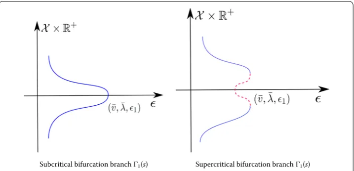
We present the plots in Figure to illustrate the first bifurcation branch or one of the solution sets to (.) schematically. Each element except (v¯,λ,¯ ) on the bifurcation branch represents a nontrivial solutions to (.). Our analysis shows that the project of each branch onto the-axis must include the interval (,).
Remark Theorem . indicates that (.) admits decreasing solutions for every small and the proof can be carried over to show that this system also admits increasing solutions. Indeed, letv(x) be a decreasing solution of (.). Then, thanks to the Neumann boundary condition,v(L–x) is also a solution, and it is increasing inx. Therefore, we can construct
Subcritical bifurcation branch(s) Supercritical bifurcation branch(s)
nonmonotone solutions by reflecting and periodically extending the monotone ones at the end points.
According to Theorem ., the shadow system (.) admits nonconstant monotone so-lutions for any small> . Therefore, from the view point of singular perturbations, we may expect that (.) also admits nontrivial solutions whenχanddare sufficiently large, and although rigorous mathematical analysis is quite technical and is out of our scope, we perform extensive numerical simulations to verify this observation in Section .
2 Nonconstant positive solutions to the shadow system
To see how bifurcation analysis is performed in [] and to introduce necessary notations and settings for our global analysis, we rewrite (.) into the abstract form
F(v,λ,) = , (v,λ,)∈X×R+×R+,
where
F(v,λ,) =
v+ (a–bλe–r(v)–cv)v L
(a–cv)e–r(v)dx–bλ L
e–r(v)dx
, (.)
andX is the Hilbert space given by (.). We remark that any nonnegative solutionvof (.) inXis a classical solution thanks to the standard elliptic embeddings.
We first collect the following facts in [] on the operatorFbefore using the bifurcation theory.
Lemma . []The operatorF(v,λ,)defined in(.)satisfies the following properties: ()F(¯v,λ,¯ ) = for any∈R+;
()F:X×R+×R+→Y×Yis analytic,whereY=L(,L);
()for any fixed(v,λ)∈X×R+,the Fréchet derivative ofFis given by
D(v,λ)F(v,λ,)(v,λ) =
v+ (a– cv–be–r(v)(λ–λvr(v)))v–be–r(v)vλ L
(bλr(v)e–r(v)–ce–r(v))v–be–r(v)λdx
; (.)
()D(v,λ)F(v,λ,) :X×R+→Y×Ris a Fredholm operator with zero index. Besides these facts, we can further show that the dimension of the null space of
D(v,λ)F(v¯,λ,¯ ) is and the following necessary condition on the null space of operator (.) holds:
ND(v,λ)F(v¯,λ,¯ ) ={}
and, in particular,
ND(v,λ)F(v¯,λ,¯ ) = span
Moreover, we can verify the following transversality condition:
and therefore the existence of nonconstant bifurcating solutions follows from the classical Crandall-Rabinowitz bifurcation theory [].
Remark We want to point out that (,a
b) is the other constant solution to (.). How-ever, it is easy to verify that Crandall-Rabinowitz bifurcation does not occur at this trivial solution. In fact, putting (v,λ) = (,ab) in (.), we see that the necessary condition (.)
We now proceed to extend the local bifurcation curves obtained in Theorem . by the global bifurcation theory of Rabinowitz [] and its developed version in []. In particular, we will only study the first bifurcation branchsince all the remaining (local) branches are unstable.
Denote the solution set of (.) by
S=(v,λ,)∈X×R×R+|F(v,λ,) = , (v,λ)= (v¯,λ)¯
and letCbe the maximal connected subset ofS¯that contains (v¯,λ,¯ ). ThenCis a closed set, and it contains (v(x,s),λ(s),(s)),s∈(–δ,δ). We show in the following lemma that all elements onCare solutions to (.) staying positive in this set.
Lemma . Assume that(.)holds.Then,for each(v,λ,)∈C,v(x) > on[,L],λ> ,
and(v,λ)is a solution of(.).
Proof We introduce the following connected set:
P= by topology arguments, and if this is done, the connectedness ofS+implies thatP
To prove thatPis closed inC, we take{(vk,λk,k)} ∈Psuch that, for some (v,λ,)∈C,
and it is well known that (.) has only the trivial solution anda
c; therefore,vkconverges to either or a
c uniformly on [,L]. Ifvkconverges to , then we can apply the Lebesgue dominated convergence theorem to the integral constraint in (.):
= lim
which is impossible. Ifvkconverges to ac, then similarly we have
= lim [,L]. Then we can apply the strong maximum principle and Hopf ’s lemma to (.) to show thatv≡ for allx∈[,L] and thereforeλ=a
b. However, this is impossible since it is easy to check that bifurcation does not occur at (,a
b). This is a contradiction, and we must
have thatv(x) > on [,L].
Remark According to Lemma . (and the forthcoming discussion), we know that the global continuumC cannot intersect with the-axis. However, we are not able to rule out the possibility that it intersects with theV-axis, that is,X×R+× {}. Details on the limiting structures are needed for this purpose. Our main results in Theorem . establish the existence of nonconstant solutions to (.) for any small, and it is out of the scope of this paper to analyze their limiting profiles.
We proceed to show that C consists of two disjoint components and each compo-nent contains solution v that is spatially monotone. Let Cu to be the component of
cor-Proof Our proof is based on the same topology arguments as in the proof of Lemma .. We introduce the following four subsets:
C
Then Lemma . holds if we can prove that
C
u⊂P+, Cl⊂P–.
We only prove the first part, and the second one can be treated in the same way. We note thatC
uis nonempty since any solution (v,λ,) of (.) near (v¯,λ,¯ ) is in the setCuthanks to (.). SinceC
uis a connected subset ofX×R+×R+, we only need to show thatCu∩P+ is both open and closed with respect to the topology ofC
u, and we divide our proof into two parts. On the other hand, we conclude fromv˜k→ ˜vinX and from the elliptic regularity theory thatv˜k→ ˜vinC([,L]). Differentiating the first equation of (.) with respect tox, we divide our discussions into the following two cases.
To prove thatC
By the same argument as before it can be easily proved thatλ˜> . We now need to show that ˜v(x) > . Again, we have from the elliptic regularity thatv˜k→ ˜vinC([,L]), and thereforev˜(x)≥,x∈(,L). Applying the strong maximum principle and Hopf ’s lemma to (.), we have that either v˜> orv˜≡ on (,L). In the latter case, we must have (v˜,λ)˜ ≡(v¯,λ), and this contradicts to the definition of¯ C
u. Thus, we have shown that˜v> on (,L), and this proves the closedness. The proof of Lemma . is complete. 3.1 Global extension of the first bifurcation branch
Finally, we study the extension of the local bifurcation branch(s), and we present a proof of Theorem ..
Proof of Theorem . According to Theorem . in [],Cusatisfies one of the follow-ing three alternatives: (A) it is not compact inX ×R+×R+; (A) it contains a point
If (A) occurs, then we can choose the complement to be
Z=
a contradiction. Therefore, only alternative (A) occurs, and Cu is not compact inX×
R+×R+.
Multiplying both hand sides of (.) bywand then integrating over (,L), we have that andλare uniformly bounded in. Then we have from the last equality that
by the same arguments as in case (A). Therefore, the claim is proved.
Now we proceed to show that the projectionCuonto the-axis is of the form (,¯] for some¯≥. We argue by contradiction and assume that there exists> such that (,)¯ is contained in this projection, but this projection does not contain any<. Then we have from the uniform boundedness ofv(x)∞and Sobolev embedding that, for each > ,vC([,L])≤Cfor all (v,λ,)∈Cu. However, this implies thatCuis compact in
X×R+×R+, which is a contradiction to alternative (A). Therefore,C
uextends to infinity vertically inX×R+×R+. This finishes the proof of Theorem ..
We have from Theorem . that there exist positive and monotone solutionsv(λ,x) to (.) for all∈(,). Ifv(x) is an increasing solution to (.), thenv(L–x) is a decreas-ing solution. Then we can construct infinitely many nonmonotone-solutions of (.) by reflecting and periodically extendingv(x) andv(L–x) atx= ,±L,±L, . . . .
4 Numerical simulations
We proceed to investigate (.) and (.) by numerical studies. Our simulation illustrates and supports our theoretical finding in the previous sections, that is, (.) admits non-trivial positive constant steady states whenχanddare large anddis small. Moreover, system (.) is able to model the well-observed phenomenon of segregation through com-petition.
According to [], in limit of largeχandd, positive solutions (u,v) of (.) over= (,L) can be approximated by those of the shadow system (.). Moreover, thanks to Theo-rem ., the boundary value problem (.) admits nonconstant solutions for any small> ; therefore, we expect the emergence of nontrivial patterns in (.) forχanddbeing large anddbeing sufficiently small. We choose the sensitivity function to beφ(v)≡ without losing much generality of our numerical studies. In the remaining part of this section, we shall numerically study the following coupled time-dependent system:
⎧
trivial solution. Moreover, we choose χ= ,d, and the initial data (u,v) = (u¯,v¯) + (., .)cosπx in all the simulations (except the initial data in Figure ). It is our goal to examine the effect ofd(or, equivalently, ofin (.)) and the domain size on the formation of nontrivial patterns in (.). Our numerics demonstrate the self-organized spatial temporal dynamics of these systems.
4.1 Simulations over one-dimensional domains
In Figure , we plot the spatial-temporal solutions to illustrate the formation of single boundary spike touand boundary layer tov. The boundary spike and layer here corre-spond to the monotone steady state obtained in Theorem .. Moreover, the numerical
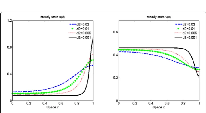
Figure 2 Formation of stable single boundary spike ofuand boundary layer ofvto (4.1) over = (0, 1).The diffusion rated2= 0.01 is chosen, whilea1=a2=b2=c1= 1,b1=c2= 2,χ= 500 andd1are
fixed and the initial data (u0,v0) are small perturbations from (u¯,v¯) as given above.
Figure 3 Smalld2supports stable steady states of (4.1) with boundary spike or layer, whered2are
simulations suggest that the spiky solutions are stable. The rigorous proof of the stability is out of scope of this paper.
According to Theorem ., (.) admits nonmonotone positive solutions for any small > ; therefore, it is natural to expect that the same holds for (.) when bothχanddare large. On the other hand, we know from our proof of Theorem . that the largedinhibits the existence of nonconstant positive solutions. Therefore, we present Figure to investi-gate the effect of smalldon the nonconstant steady states to (.). Asdtends to zero, the boundary spike shifts to the boundary with its magnitude increases. However, rigourous analysis of these spiky solutions is quite challenging and is out of the scope of this paper.
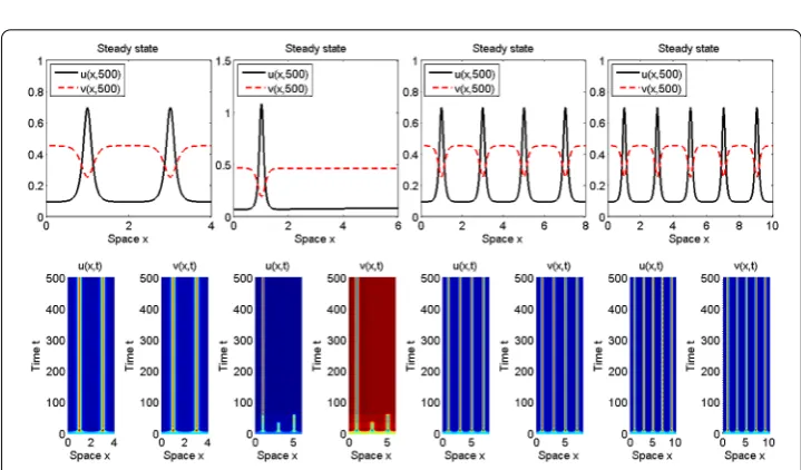
Figure 4 Formation of stable interior spike ofuand interior layer ofv.All the system parameters and initial data are as in Figure 2 except that the interval length isL= 2.
Thanks to the Neumann boundary conditions, we can construct single- and multi-interior spikes for (.) by reflecting and periodically extending the single boundary spike at the end points. This is numerically demonstrated in Figure .
In Figure , we continue to examine the effect of large interval on the formation of multi-spikes in (.). We observe the reflection and periodic extension of multi-spikes over interval withL= to thoseL= andL= . However, we may expect steady states with three spikes whenL= , admitting a single interior instead. We are motivated to study the dynamics of such an irregular pattern observed in Figure whenL= . To do so, we selectL= and plot in Figure the profile ofu(x,t) for specifically chosen times. We observeu(x,t) develops with multispikes which are meta-stable, the stability of which is destroyed at time
Figure 6 Evolution and dynamics ofu(x,t) over (0, 16).The system parameters are chosen as in Figure 2. We observe that solutions with eight spikes emerge att≈5 and develop into metastable pattern, which is destroyed att≈46. After that, interior spikes merge and develop into a single spike, which becomes stable finally.
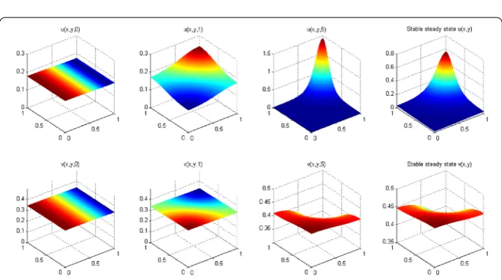
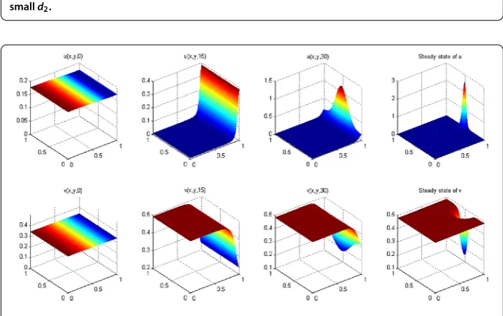
Figure 8 Qualitative behavior of stable steady states with a single boundary spike in the limit of smalld2.
Figure 9 Evolution and formation of single boundary spike that is not located at the corner.The initial data are constant inxbut constant iny.
t≈. Then we observe the merging and disappearing of the interior spikes, and finally
u(x,t) develops into a single interior spike afterwards. 4.2 Simulations over two-dimensional domains
spatial-Figure 10 Stable steady states with both interior and boundary spikes over varying squares.
temporal of these spikes is an interesting but also quite demanding question that we can study in the future.
Competing interests
The authors declare that they have no competing interests.
Authors’ contributions
Both authors read and approved the final manuscript and contributed equally to the writing of this paper. Numerical simulations are mainly due to YZ, and the analysis is mainly due to LX.
Author details
1School of Securities and Futures, Southwestern University of Finance and Economics, Chengdu, 611130, China.2College
of Mathematics and Statistics, Guangdong University of Finance and Economics, Guangzhou, Guangdong 510320, China. 3College of Mathematics and Statistics, Shenzhen University, Shenzhen, Guangdong 518060, China.
Acknowledgements
YZ supported by Department of Education, Sichuan (15ZB0473). LX supported by Guangdong Natural Science Foundation (2015A030313623) and Guangdong Training Program for Young College Teachers (YQ2015077).
Received: 5 October 2016 Accepted: 6 January 2017
References
1. Wang, Q, Gai, C, Yan, J: Qualitative analysis of a Lotka-Volterra competition system with advection. Discrete Contin. Dyn. Syst.35, 1239-1284 (2015)
2. De Mottoni, P, Rothe, F: Convergence to homogeneous equilibrium state for generalized Volterra-Lotka systems with diffusion. SIAM J. Appl. Math.37, 648-663 (1979)
3. Kishimoto, K, Weinberger, H: The spatial homogeneity of stable equilibria of some reaction-diffusion systems in convex domains. J. Differ. Equ.58, 15-21 (1985)
4. Matano, H, Mimura, M: Pattern formation in competition-diffusion systems in nonconvex domains. Publ. Res. Inst. Math. Sci.19, 1049-1079 (1983)
5. Mimura, M, Ei, S-I, Fang, Q: Effect of domain-shape on coexistence problems in a competition-diffusion system. J. Math. Biol.29, 219-237 (1991)
6. Mimura, M, Kawasaki, K: Spatial segregation in competitive interaction-diffusion equations. J. Math. Biol.9, 49-64 (1980)
7. Mimura, M, Nishiura, Y, Tesei, A, Tsujikawa, T: Coexistence problem for two competing species models with density-dependent diffusion. Hiroshima Math. J.14, 425-449 (1984)
8. Shigesada, N, Kawasaki, K, Teramoto, E: Spatial segregation of interacting species. J. Theor. Biol.79, 83-99 (1979) 9. Choi, YS, Lui, R, Yamada, Y: Existence of global solutions for the Shigesada-Kawasaki-Teramoto model with weak
cross-diffusion. Discrete Contin. Dyn. Syst.9, 1193-1200 (2003)
10. Kuto, K: Limiting structure of shrinking solutions to the stationary Shigesada-Kawasaki-Teramoto model with large cross-diffusion. SIAM J. Math. Anal.47, 3993-4024 (2015)
11. Lou, Y, Ni, W-M, Yotsutani, S: On a limiting system in the Lotka-Volterra competition with cross-diffusion. Discrete Contin. Dyn. Syst.10, 435-458 (2004)
13. Kuto, K, Tsujikawa, T: Limiting structure of steady-states to the Lotka-Volterra competition model with large diffusion and advection. J. Differ. Equ.258, 1801-1858 (2015)
14. Crandall, MG, Rabinowitz, PH: Bifurcation from simple eigenvalues. J. Funct. Anal.8, 321-340 (1971)
15. Ni, W-M, Polascik, P, Yanagida, E: Monotonicity of stable solutions in shadow systems. Transl. Am. Math. Soc.353, 5057-5069 (2001)
16. Rabinowitz, PH: Some global results for nonlinear eigenvalue problems. J. Funct. Anal.7, 487-513 (1971) 17. Shi, J, Wang, X: On global bifurcation for quasilinear elliptic systems on bounded domains. J. Differ. Equ.246,