An Energy and Application Scenario Aware Active RFID Protocol

(1)

Volume 2010, Article ID 432938,15pages doi:10.1155/2010/432938

Research Article

An Energy and Application Scenario Aware Active RFID Protocol

Bj¨orn Nilsson,

1, 2

_{Lars Bengtsson,}

1, 3

_{and Bertil Svensson}

1

1_{Centre for Research on Embedded Systems (CERES), Halmstad University, 30118 Halmstad, Sweden} 2_{Research Department, Free2move AB, 302 48 Halmstad, Sweden}

3_{Department of Computer Science and Engineering, Chalmers University of Technology, 412 96 Gothenburg, Sweden}

Correspondence should be addressed to Bj¨orn Nilsson,bjni@hh.se

Received 11 July 2010; Accepted 28 November 2010 Academic Editor: A. Vasilakos

Copyright © 2010 Bj¨orn Nilsson et al. This is an open access article distributed under the Creative Commons Attribution License, which permits unrestricted use, distribution, and reproduction in any medium, provided the original work is properly cited. The communication protocol used is a key issue in order to make the most of the advantages of active RFID technologies. In this

paper we introduce a carrier sense medium access data communication protocol that dynamically adjusts its back-oﬀalgorithm to

best suit the actual application at hand. Based on a simulation study of the eﬀect on tag energy cost, read-out delay, and message

throughput incurred by some typical back-oﬀalgorithms in a CSMA/CA (Carrier Sense Multiple Access/Collision Avoidance)

active RFID protocol, we conclude that by dynamic tuning of the initial contention window size and back-oﬀinterval coeﬃcient,

tag energy consumption and read-out delay can be significantly lowered. We show that it is possible to decrease the energy consumption per tag payload delivery with more than 10 times, resulting in a 50% increase in tag battery lifetime. We also discuss the advantage of being able to predict the number of tags present at the RFID-reader as well as ways of doing it.

1. Introduction

1.1. Background. Emerging technologies, like printed batter-ies and the continuous advancements in CMOS-ASIC (Com-plementary Metal Oxide Semiconductor-Application Spe-cific Integrated Circuit) fabrication and antenna technolo-gies, cast new exciting light onto the established technology of Radio Frequency IDentification (RFID). The mentioned developments have made it possible to expand the usage of RFID and narrow the span between diﬀerent flavors of RFID technologies. The RFID technique is used to remotely and wirelessly identify a device namedtransponder (ortag) by using an interrogator (orreader). The tag has a unique identity used to identify the object it is attached to. The RFID technology can be divided into two main categories, passive RFID and active RFID. This work investigates the possibilities of defining an active RFID protocol that is paving the way for diﬀerent applications without deteriorating the performance regarding tag lifetime and read-out delays. We argue that, for this to be possible, the protocol must be adaptable to the specific application scenario at hand. In a previous paper [1] we have introduced such a protocol and demonstrated the possible gains in tag energy consumption and read-out delay.

In the current paper we first show the great advantages of using carrier sense; we then review the principle and design of the adaptable protocol, and finally present how to get maximum advantage of such a protocol.

1.2. Paper Outline. The outline of this paper is as follows. In Section 2, RFID systems and related research work are presented, and in Section 3 we show the impact of using carrier sense in active RFID protocols.Section 4introduces the suggested, application sensitive, active RFID protocol which is built on the idea of adaptively choosing the best back-offalgorithm parameters.Section 5shows the setup for the simulation that we use for simulating the behavior of five different back-offalgorithms and describes the protocol and the five algorithms. Then Section 6 shows simulation results.Section 7shows optimization in regards to the delay or to the power consumption.Section 8explores the design space.Section 9describes the suggested dynamic active RFID Medium Access Control (MAC) protocol. InSection 10we discuss different ways of estimating the number of tags in an active RFID scenario as an introduction to future work.

(2)

2. RFID Systems

2.1. RFID Application Scenarios. Automation in logistics has driven the development of RFID in the past years. Scenarios for RFID [2] appear, for instance, in the logistics chain, tracking goods from the producer to the consumer, depicted inFigure 1, where the goods can be one single product or up to several hundred products on a single pallet; seeFigure 2. Items must be identified with short delay by the RFID-reader when, for example, they are passing an RFID-reader on a vehicle with high speed. In this realm, RFID could also be used for automatic inventory of the stock in a warehouse, where the reading delay is not critical but where there is a huge amount of tagged goods to identify.

In some applications the physical constraints (e.g., radi-ated power from the reader) of the RFID-system set the limit of functionality (e.g., limits the reading range). The RFID-reader in a scenario with a fork lift passing the RFID-reader closely needs only a small amount of radiated energy, due to the short distance, but needs fast readings due to the high vehicle velocity. For a scenario with a large warehouse, and thus long distances, the reader needs to radiate higher amount of energy—unless many RFID-readers are deployed, yielding the well-known drawback with the “multi-reader problem” which deteriorates readability; however this scenario has no hard read-out time requirements.

2.2. Passive and Active RFID. There are three main types of RFID: passive RFID, active RFID, and semi-RFID. The “semi” means that the tags are partly battery powered to assist a more complex processor core that boosts functionality compared to passive RFID.

The most common RFID technology today is passive RFID. The tags have no energy source of their own; instead they are powered by the reader’s magnetic or electromagnetic field which is converted to electrical power. Although this enables low-cost tags the main drawbacks are: (1) the limited working distance between reader and tag, (2) the high transmitted reader energy required; and (3) the fact that sensor readings and calculations are not possible when there is no reader in the vicinity to power the tags.

In active RFID the working distance can be much longer (a few hundred meters, set by the link budget). Active RFID tags, having their own power sources, can use higher transmit power and receivers with higher sensitivity. Other benefits are sensor measurements, complex calculations, and storage even when there is no reader in the vicinity of the tag. The possible rate of detecting tags is dependent on a combination of range and output power from the reader. For scenarios which need fast detection of tags this implies dense readings close to the reader in passive RFID (the reader powers the tags only from a short distance, typically a few decimeters). Active RFID systems can spread the readings in the time domain and in distance from the reader and therefore oﬀer a higher throughput of tag readings.

2.3. Today’s Standards and Protocols. Much work has been done for standardization of passive RFID, such as

Producer

Transporter

Wholesaler

Transporter

Retailer

Customer

Local tracing

Global tracing

Automated inventory

Proof of delivery

Inventory

Product status

Figure1: Logistics chain supervision.

Figure2: Diﬀerent application scenarios requiring diﬀerent

read-out delay and throughput to be eﬃcient.

the EPCglobal standards development [3]. The majority of active RFID protocols are proprietary. However, some exist-ing standards used in WLAN and Zigbee are currently beexist-ing used in active RFID applications despite their disadvantages regarding tag price and battery life-time [4].

The standard ISO 18000-7 [5] defines the air interface for a device acting as an active tag. Its purpose is to provide a common technical specification for active RFID devices. An implementation [6] of ISO 18000-7 shows good readability but rather poor performance for dense tag applications, due to the arbitration technique used and the long time to retrieve tag information. Yoon et al. [7] propose a modified tag collection algorithm based on slotted ALOHA that complies with the ISO 18000-7. This modified algorithm allows choosing an optimum slot size for receiving one tag response according to its data processing capabilities.

(3)

increase throughput and minimize read-out delay. However, this is not directly applicable to active RFID due to its different nature (this is further elaborated on inSection 4.1). Protocol design should address the different needs for the different applications scenarios. Some application, needs short read-out delays but some do not; having this in mind when designing the protocol, it is possible to reduce the tag power consumption and thereby increase tag battery life-time.

2.4. Related Research Work on Active RFID Protocols. There are several companies developing systems for active RFID, but no agreement exists of a worldwide standard that fits a large variety of applications scenarios.

Research done by Bhanage and Zhang [8] to enable a power eﬃcient reading protocol for active RFID shows interesting results. Their idea is to reduce information sent in the network and also to reduce the energy used to detect collisions by enabling smart sequencing in real time. The Relay MAC protocol proposed yields better throughput and energy conservation than a conventional binary search protocol. The disadvantage of the Relay MAC protocol is that the reader coordinates the reading sequence, which means that when a load with new ID-tagged goods arrives at a reading spot, the reading sequence has to be reinitialized.

Li et al. [9] suggest a DCMA (Dual Channel Multiple access) protocol for active RFID where long information packets are used. One channel is used for control and the other for data. Thus, when new tags enter the system on the control channel, they will not collide with tags scheduled on the data channel. This is said to reduce the power consumption but the effect on delay or throughput of the active RFID system is not reported. Every tag starts by doing an exponential back-offand then starts to send. The reduced power consumption is explained to be due to the use of a control channel and the tag power-down-mode during the back-off. The authors report simulations with up to 20 tags, a rather small amount. They claim a life-time of five years when the battery capacity is 950 mAh and 100 readings are made per day. Nothing is mentioned about how many tags that were used in the active RFID-system when achieving the five years of life-time.

An interesting way of reducing power is described by Chen et al. [10]. Instead of the tag waking up periodically, a sensor-based wake-up is used. Their experiments show that, with a sensor-enhanced active RFID system, the battery lasts twice as long in comparison to a system without any embedded sensors.

With focus on waking a tag by using low energy, Hall et al. [11] have constructed a “turn-on circuit” in standard CMOS technology based on a Schottky barrier diode. Calculations of the usable “turn on” range (using a favorably oriented antenna with 6 dB of gain an operating frequency of 915 MHz, and output power of 1 W) give a theoretical operating range of 117 m.

Jain and Das [12] have developed a CSMA-based (Carrier Sense Multiple Access) MAC protocol [13] to avoid collisions in a dense active RFID network. Results from evaluations

show that it has superior performance compared to a randomized protocol with regard to readability (probability that many readers read the same tag when the tag is in the vicinity of several readers at the same time) and time per tag read.

A stochastic anticollision algorithm, the DFSA algorithm (Dynamic Framed Slotted ALOHA) is investigated by Leian and Shengli [14]. They show that, in a slotted ALOHA-based anticollision RFID system, maximum throughput is achieved when the number of slots is the same as the number of tags. For estimation of the number of tags, two methods (based on a ternary feedback model) are presented and demonstrated.

A hybrid TDMA (Time Division Multiple Access) MAC protocol is proposed for active RFID by Xie and Lai [15]. The protocol is contention based for high density tag conditions. The tag contends, by using Rivest’s Pseudo-Bayesian algorithm, to get a communication slot and then stays synchronized with the reader with the TDMA protocol. For active RFID systems using transmit-only tags, Mazurek [16] proposes a DS-CDMA (Direct Sequence Code Division Multiple Access) protocol to improve tag recognition rate. The tags do not need to be synchronized with the reader, which keeps the tag design simpler. Sim-ulations show that the proposed DS-CDMA outperforms the classical narrow band Manchester-coded RFID/ALOHA when comparing probability of tag detection.

3. Active RFID and Carrier Sense

Carrier sense (CS) is used to avoid collisions in the radio channel. Using the carrier sense functionality has an advan-tage as long as the energy consumption for the sense action is held low. Simulation results [17] depicted in Figures3,4, and 5 show comparisons between using and not using CS in the same type of tag transmit first ALOHA protocol. For instance, inFigure 3 the CS protocol has 2.3 times higher throughput when there are 400 tags and 5 times higher throughput in the case of 1000 tags. Every tag wakes up during a cycle (the cycle time is set to one second in this case), at a time which has a uniform random distribution. The CS protocol, which is the top curve inFigure 3, shows highest throughput and heads towards maximum channel utilization (which theoretically is 556 tags/second). The throughput would of course decrease if propagation delays increase (and are of great magnitude) as shown by Rom and Sidi [13]. In this simulation the propagation delay is set to zero but for real cases it is less than 200 nanosecond and is a small fractional part of the CS (128 microsecond), resulting in a very low impact on the propagation delay.

(4)

0

0 500 1000 1500 2000 2500 3000

Number of tags Throughput

Non-CS CS

Figure3: Throughput: number of tags read per second.

lifetime, presented in Figure 5, reveals the much lowered energy consumption when using CS.

4. The Adaptive Protocol

The medium access protocol modeled in our study is a contention-based nonpersisting carrier sense multiple access protocol with collision avoidance (CSMA/CA) using a nonslotted channel; see Figure 6. It supports both cyclic awakening RFID systems as well as wake-up radio based. (A cyclic awakening system is when the tags wake up periodically trying to deliver their payload regardless if there is an RFID reader or not. The wake-up radio-based tags are equipped with a circuit that can sense if there is an available RFID-reader and thus know when to deliver its payload.)

The reader continuously broadcasts messages containing three parameters: (1) channel: what frequency the tag should transmit its payload on; (2)ICW(Initial Contention Window): the time period during which all tags must try to do their first transmission attempt; and (3) a coeﬃcient (explained later). The tag uses the information to select a stochastically evenly distributed initial back-oﬀ time (t0,Figure 8) during theICWand calculates the subsequent

back-offtimes using the appropriate algorithm and coeffi -cient. After the initial back-offtime the tag performs a carrier sense (CS) to detect if the radio channel is free to use. If the channel is occupied, the tag performs a new back-off. Eventually the data packet (200 data bits) will be successfully delivered to the reader, and the tag enters sleep mode.

The key feature in our active RFID protocol is the possibility to adapt the back-off algorithm to different application scenarios. When tailoring an active RFID pro-tocol for different application scenarios we need to define the most important application constraints. These have been identified to be the energy consumption, the message

0

0 500 1000 1500 2000 2500 3000

Delay

Number of tags Non-CS

CS

Figure4: Delay: average time to read all available tags (the cycle time is set to 1 second).

0

0 500 1000 1500 2000 2500 3000

Number of tags Draining a battery with a tag

Non-CS CS

Figure5: Lifetime of a tag powered CR2032 (150 mAh) lithium cell. The non-CS curve is extrapolated above 800 tags.

throughput, and the out delay requirements. The read-out delay is the time taken from when the tag is addressed until it delivers its data.

4.1. Related Work on Back-Off Algorithms in Wireless Net-works. Some research work has been published on how to achieve higher efficiency (fewer collisions on the radio channel) in the IEEE 802.11 standard by applying different back-offstrategies.

(5)

Sleep Initial

back-off

back-off Sleep,

reader wakes it

RFID-reader available

RFID-reader not available

TX: Transmit CS: Carrier Sense Ack: Acknowledge RFID-reader not available

Time

TX Ack

CS

Sleep Initial

back-off Sleep,

reader wakes it CS TX Ack

Back-off 1

Back-off 1 Sleep,

reader wakes it CS

Initial _CS _CS

Back-off 2 CS TX Ack Sleep

Tag 1

Tag 2

Tag 3

Figure6: Tags delivering their payload packets to a reader.

relies on the number of neighbor nodes. The required minimum contention window is shown to be proportional to the number of neighbors. Experiments also show that the NBA shows better behavior than the often used Binary Exponential Back-oﬀ.

Jayaparavathy et al. [19] suggest that the back-oﬀtime for each contending node can be modified by retrieving information obtained from transmitting stations (delay from the contending nodes) thereby getting higher throughput and shorter delays.

Bhandari et al. [20] present simulation results that show that, by using binary slotted exponential back-off, the throughput and delay are sensitive to the initial back-off window size, the payload size, and the number of stations in the network. The results can be used to decide the protocol parameters for optimum performance under different loading conditions.

An algorithm in which exponentially increasing/de-creasing (EIED) back-oﬀ is used is presented by Song et al. [21].

An alternative back-offpolicy, called theμ-law or the step function, can outperform the exponential back-off, as shown by Joseph and Raychaudhuri [22]. These back-offalgorithms consider slower reduction of the back-offtime in the initial phase of back-offand then a more rapid reduction.

A distributed back-off strategy to achieve lower power consumption has been studied by Papadimitratos et al. [23], claiming 154% more data bits per unit energy consumed in the network. This is done by determining the back-offperiod for each transmitting node based on the node’s wireless link quality. The better the link quality is the shorter back-off period is used.

The described related work on wireless networks is not directly adaptable to active RFID due to its diﬀerent nature. In active RFID, short messages from a large number of tags must be passed on to the reader with short delay and with very low energy consumption. The reader-tag communication does not need to establish a continuous communication link as in other wireless networks.

Algorithms Constant Linear Linear modulus Exponential Exponential modulus

Number of tags

Coeﬃcient

ICW

Iterated 100 times to get average 1–100

Step 1 50–1050 tags Step 100 tags

100–4900 ms Step 300 ms

Figure7: The simulation procedure.

5. Simulation Setup

Through simulations, the energy consumption and read-out delays incurred by the five different back-offalgorithms and their back-offcoefficients and Initial Contention Windows have been determined. Here we present the physical con-straints of the radio channel, the simulation method, and the simulation model.

(6)

Exponential mod (5) Exponential Linear mod (5)

Linear Constant B3 B4 B5 B6

Time B8

B8

B9

B9 B1

B1

B2 B3

B1

B1 B2

B2 B3

B3

B1 B2 B3

B4 B5

B5

B5 B6

B6

B6 B7

B7

B7 B10 B11

B4

B4 B2

ICW

ICW t0

t0

Figure8: Types of back-oﬀalgorithms: constant, linear, linear modulus, exponential, and exponential modulus. The arrow ending at time

to (randomly chosen by each tag in the range of theICW) is the initial back-oﬀ, then increasing B-numbers show successive back-oﬀs.

Shadowed parts show randomness in the back-oﬀtime which is added to eachTi.

The times for the transceiver to switch between the diﬀerent states (TX, RX, CS) are neglected because these times typically are much shorter than the packet transmission time.

The active RFID system modeled is built using the physical constraints of a commercially available transceiver [24] working in the 2.45 GHz ISM band with a bit rate of 250 kbit/second. It has a working range of more than 50 m calculated with free space propagation attenuation. The maximum output power is 0 dBm, the receiver sensitivity is −90 dBm, and the channel bandwidth is 1 MHz.Table 1

shows power and time requirements for the transceiver to do a CS, a TX (200 bits), and an ACK (200 bits).

5.2. Simulation Method and Model. All simulations are done using Matlab and begin with a population of 50 tags available to the reader. Simulations are then done for an increasing number of tags until reaching 1050. All tags are assumed to wake up simultaneously when there is a reader in the vicinity, without consuming any energy and in zero time. Every tag has to deliver its payload packet and receive an acknowledge packet before the simulation ends. Both the payload and the acknowledge packets are 200 bits long.Figure 7depicts the simulation procedure.

5.3. The Back-OﬀAlgorithms. The back-oﬀalgorithms sim-ulated are: constant (1), linear (2), linear modulus (3), exponential(4),andexponential modulus(5). The following

Table1: Power and time constraints when the tag is in diﬀerent states.

Mode Power consumption [mW] Duration (ms)

Carrier Sense 57.0 0.128

Transmit 42.0 1.6

Receiving an ACK 57.0 2.0

Sleep 0.011 varies

equations describe the five algorithms. The behaviors of the algorithms are depicted inFigure 8:

ti+1=ti+C·Tslot, (1)

ti+1=ti+L·i·Tslot, (2)

ti+1=ti+L·(imodr+ 1)·Tslot, (3)

ti+1=ti+E·2i·Tslot, (4)

ti+1=ti+E·2(imodr)·Tslot. (5)

Here, C, L, and E are coeﬃcients, i = 0, 1, 2, is the back-oﬀsequence number, andti is the absolute time

(7)

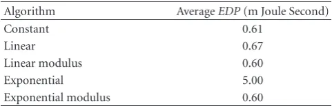
Table2: AverageEDP.

Algorithm AverageEDP(m Joule Second)

Constant 0.61 In our simulations we used r = 5.Tslot refers to the time

to do one TX and one Ack.

Theconstant,linear, andexponentialback-oﬀalgorithms are simulated with their coeﬃcients,C,L, andErespectively, stepped in the range from 1 to 100. The variable ICW is in the range from 100 milliseconds to 4900 ms in steps of 300 ms. The results from the simulations are the delay and the number of performed carrier senses. This is repeated 100 times, after which an average value is calculated.

Each tag makes a first initial random back-oﬀin theICW. On waking up, the simulated tag does a carrier sense, and if the radio channel is free (no other tag, nor the reader, is doing a transmission), a payload packet is transmitted to the reader. If the radio channel is occupied the tag makes a new back-oﬀ. A small random time is also added to prevent tags from trying to communicate periodically at the same time (shown as shadowed inFigure 8). This randomness is a time between 0 and 7.2 milliseconds (which is the time to do two RXs and two TXs using the modeled transceiver). Hidden terminals (tags within range of the reader but out-of-range of each other) are handled via the ACK protocol used (the tag retransmits its message until it receives an ACK from the reader and then sleeps for the rest of the simulation).

6. Results

Applications using active RFID need to be optimized both for long lifetime and for short delays. Unfortunately, these two goals are in conflict with each other, so a trade offis necessary. In this section the performance of each of the algorithms is analyzed by extracting data from simulations and calculating the tag energy consumption and the tag read out delay. The algorithms are then compared over a large application space (finding, for different numbers of tags, the minimum energy consumption and minimum read out delay possible by choosing the best coefficient and the best ICW).

6.1. Energy, Delay and EDP. The simulation results are presented in the form of: (1) Energy, which is the energy consumption per delivered payload packet; (2) Delay, which is the read out delay; and (3) Energy Delay Product (EDP= Energy×Delay) [1,25], a “goodness” value used for overall comparison of algorithms.

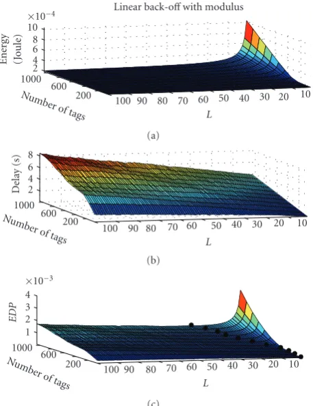
In Figures9,10,11,12and13 Energy, Delay, andEDP are shown as a function of the number of tags and the coeﬃcient for the diﬀerent algorithms. Both energy and

delay also depend on the ICW, but this is not shown in the figure. Instead, the minimum values, when theICW is varied, are presented; see (6). The EnergyS is the energy

in average required by a tag for doing all necessary carrier senses, transmitting one payload packet and receiving one acknowledge packet. The read-out delay, DelayS, is the

average time until every available tag has delivered one payload packet:

Figure 9 shows results from simulation of the constant back-oﬀalgorithm. The energy diagram ofFigure 9shows the energy consumption in Joule for a tag in delivering a payload to the reader. A maximum in energy consumption can be seen when there are 1050 tags and the coeﬃcientCis small.Figure 9(b)shows the Delay in seconds. The longest delay exists when there are 1050 tags and a largeC, and then successively a somewhat shorter delay when decreasingC.

To compare the algorithms the EDP metric has been used. The EDP, (7), is the minimum of the product of energy and delay for each number of tags and each coeﬃcient when varying theICW, shown in Figures9(c),10(c),11(c),

12(c)and 13(c). For each number of tags there also exists a minimumEDP(8) and these values are presented as dots connected with a white line in theEDPgraph. For instance, when there are 550 tags in the vicinity of the reader,EDPhas a minimum whenC=15:

The ICW values are extracted from the simulations separately and are not shown in the diagrams.

To compare how the algorithms behave under varying loads an averageEDPvalue has been calculated (9).nis the incremental factor used to calculate the number of tags, and EDPminis the lowestEDPpossible with that number of tags:

AvrEDP= 10

n=0EDPmin(n·100 + 50)

11 . (9)

The averageEDPis shown inTable 2. The data shows that four of the algorithms (const, lin, lin-mod, exp-mod), on average, perform similarly regarding the averageEDPmetric. The exception is the exponential algorithm without modulus which shows a much higher value.

7. Optimization

(8)

2

Figure9: Simulation results for constant back-oﬀtime: min Energy Consumption (a), min Delay (b), and Energy-Delay Product (c) as

a function of the coeﬃcientC, and the number of tags.

application scenarios we need to define the most important application constraints. These have been identified to be the energy consumption, the message throughput and the read-out delay requirements. The read-out delay is the time taken from when the tag is addressed until it delivers the data.

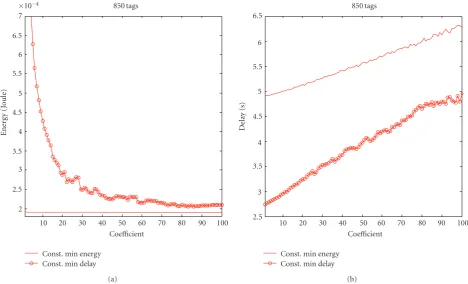
Applications using active RFID need to be optimized both for long lifetime and for short delays. Unfortunately, these two goals are in conflict with each other, so a trade oﬀ is necessary. Conclusions show that it is possible to implement only one of the proposed algorithms by choosing the appropriate ICW and the appropriate constant to be able to adapt to diﬀerent application constraints. Figure 14

shows the situation when 850 tags are in the vicinity of the reader and using the constant algorithm. The figure shows that there is a trade-oﬀ between delay and energy consumption by changing the coeﬃcient and the ICW.

Figure 14(a)shows, as a line at the bottom of the diagram, the minimum energy consumption of a tag for the constant algorithm. The lines with small circles are the corresponding energy consumption values when theICWhas been chosen for the minimum delay.Figure 14(b)shows the minimum delay (line with circles). In this diagram the plain line shows what the delays are when using the minimum energy.

Figure10: Linear back-oﬀalgorithm.

2

Linear back-oﬀwith modulus

Num

(9)

2

Figure12: Exponential back-oﬀalgorithm.

It is shown that minimizing the delay will increase the energy consumption by more than 8 times, and that minimizing the energy consumption will increase the delay by 2.3 times. The conclusion is that one can choose to minimize with regard to energy consumption or delay or find a compromise. To achieve an energy eﬃcient protocol one should dynamically select the coeﬃcient as well as theICW, depending on the application scenario.

8. Exploring the Design Space

For a specific application scenario, the appropriate ICW and coefficient must be identified. Table 3 shows, for the constant back-offalgorithm, how to choose the ICW and the coefficient and how much energy is needed for a tag to transmit a payload packet to the reader. The table data is extracted from simulation results.

For example, assume that the application normally uses 250 tags and that they are in range of the reader for 3 seconds. In this case a delay of 2500 ms is chosen (nearest to 3 seconds and still not over 3 seconds), and the number of tags is chosen from the second column, 250 tags. Now the ICW is read out as 2500 ms and the coeﬃcient is set to 2. The average energy consumption for a tag to transmit its payload is 186μJ. The empty areas in the table represent situations where it is impossible to have all tags deliver their payload within the given time. The upper row also includes the minimum delay with that specific amount of tags. For example, when there are 50 tags, the minimum delay for all tags to deliver a payload is 211 ms. By observing the region near the empty area one can conclude that operating near minimum delay (read tags fast) increases the energy consumption.

WhileTable 3is only for one of the algorithms (constant) with varying number of tags, Tables 4 and 5 compare all

2

Exponential back-oﬀwith modulus

Nu

Figure13: Exponential back-oﬀalgorithm with modulus.

(10)

2 2.5 3 3.5 4 4.5 5 5.5 6 6.5 7

×10−4

Energ

y

(J

o

ule)

10 20 30 40 50 60 70 80 90 100 Coeﬃcient

850 tags

Const. min energy Const. min delay

(a)

2.5 3 3.5 4 4.5 5 5.5 6 6.5

850 tags

Dela

y

(s)

10 20 30 40 50 60 70 80 90 100 Coeﬃcient

Const. min energy Const. min delay

(b)

Figure14: The energy-delay trade oﬀin the case of 850 tags and the constant algorithm. (a): Energy consumption as a function of the

back-offcoefficient. (b): Delay as a functions of the back-offcoefficient. “Lines with circles” show when theICWhas been selected in order

to minimize the delay. The “plain” lines show when theICWhas been selected in order to minimize energy.

FromTable 5it is possible to extract information on how much better it is to use an adaptive protocol compared to a non-adaptive. If not using an adaptive protocol the worst case scenario has to be assumed, which is when there are a vast number of tags that need to be read fast (column 1 at a read-out delay of 3825 ms giving us an energy consumption of 2052μJ). If the application accepts a longer read-out delay it is possible to adapt the protocol and save energy. Relaxing the constraint on the read-out delay to 7000 ms gives an energy consumption of 195μJ, thus decreasing the energy consumption per tag payload delivery more than 10 times.

9. The Suggested Dynamic Active

RFID MAC Protocol

The MAC protocol functions according to the protocol described in Figures6and8. Tags in range of the reader are awakened by a broadcast message (a continuously repeated beacon signal) from the reader which includes what channel they should identify themselves on, and which coeﬃcient and ICWto use.

As discussed in the previous section it is possible to choose one of the algorithms and still meet the delay and energy constraints. Tags then only need to implement, e.g., the constant algorithm. The reader adapts the coeﬃcient and ICW based on known application context and on history information from previous read-outs. Should these values

be too hard to extract (because, for example, the number of tags is totally unpredictable) the worst-case parameters should be used (minimum delay and maximum number of tags). The appropriate values for theICWand coeﬃcient (C) for the constant back-oﬀalgorithm are then to be chosen dynamically fromTable 3(note that for RFID-systems where

Table 1values not are applicable, Tables3–5values need to be regenerated).

To obtain the tag battery life time in days as functions of the number of tags and the required delay see Table 6. Assumed is a 3-Volt lithium tag battery (CR2032) with a capacity of 150 mAh. The energy values from Table 3 are used. It is assumed that each tag delivers one payload, packet once per minute. When a tag has delivered its payload it goes to sleep until the next read. The “sleep” power value fromTable 1is therefore added when calculating the energy values inTable 6. In the case when the tag stays in sleep all the time the battery will last for 1705 days.Table 6 reveals that the tag battery lifetime varies from a minimum value of 961 days (450 tags, 1.7 seconds delay) to a maximum value of 1452 days (50 tags, 6 seconds delay). To adaptively be able to choose protocol parameters,Table 6shows that the lifetime can be increased by more than 50%.

10. Estimating the Number of Tags

(11)

Table3: TheICWand the coeﬃcient values,C, giving lowest energy consumption (Energy) when choosing a specific delay and a specific number of tags for the constant algorithm.

Number of tags (Constant) Delay

(ms)

50

(Min delay=

211 ms)

250

(Min delay=

935 ms)

450

(Min delay=

1659 ms)

650

(Min delay=

2381 ms)

850

(Min delay=

3103 ms)

1050

(Min delay=

3825 ms)

250

ICW= 100 ms C=4

Energy=

208μJ

500

400 ms 13

186μJ

1000

1000 ms 400 ms

1 3

182μJ 324μJ

1700

1600 ms 1600 ms 1000 ms

35 10 1

182μJ 191μJ 529μJ

2500

2500 ms 2500 ms 2200 ms 2200 ms

40 2 13 1

182μJ 186μJ 199μJ 348μJ

3200

3100 ms 3100 ms 3100 ms 3100 ms 2200 ms

17 26 11 4 2

182μJ 184μJ 190μJ 203μJ 521μJ

4000

4000 ms 4000 ms 4000 ms 3700 ms 3700 ms 3400 ms

75 4 1 20 10 2

182μJ 183μJ 187μJ 194μJ 211μJ 394μJ

5000

4900 ms 4900 ms 4900 ms 4900 ms 4900 ms 4900ms

19 2 17 12 6 4

181μJ 183μJ 185μJ 188μJ 194μJ 207μJ

6000

4900 ms 4900 ms 4900 ms 4900 ms 4900 ms 4900ms

19 2 99 93 67 42

181μJ 183μJ 185μJ 187μJ 192μJ 200μJ

a protocol that is energy and performance eﬃcient over the entire imagination space seems to be a nonimaginable task. In order to use a protocol that can adapt to the application scenarios at hand we need information that characterizes the current circumstances and requirements.

As mentioned earlier, one issue is to predict the number of tags available to the RFID-reader. For applications where the number of tags is highly predictable, statistic calculations can be used, for example, a normal distribution averaging (over time) window. Kheiri et al. [26] use a method where they, by reading tags during a period of time can estimate the total number of tags. The method used to model the number of tags is inter-arrival times for a renewal process. This could be applicable to our proposed back-oﬀprotocol.

A method suggested by Floerkemeier [27] shows good performance compared to existing approaches by predicting the tag population using Bayesian broadcast strategies.

The transmission control scheme is based on framed ALOHA and makes no restrictive assumption about the distribution of the number of tags close to the reader.

(12)

Table4: TheICWand the coeﬃcient values,C,L, andE, giving lowest energy consumption (Energy) when choosing a specific delay, 50 tags,

and the diﬀerent algorithms.

50 Tags Delay

(ms)

Constant

(Min delay=211 ms)

Linear

(Min delay=279 ms)

Linear modulus

(Min delay=225 ms)

Exponential

(Min delay=450 ms)

Exponential modulus

(Min delay=276 ms)

211

ICW=100 ms

C=1

Energy=236μJ

225

100 ms ICW=100 ms

2 L=1

221μJ Energy=220μJ

279

100 ms ICW=100 ms 100 ms ICW=100 ms

6 L=1 3 E=1

203μJ Energy=209μJ 202μJ Energy=203μJ

450

400 ms 400 ms 400 ms ICW=400 ms 400 ms

8 4 5 E=1 1

186μJ 186μJ 186μJ Energy=186μJ 187μJ

1000

1000 ms 1000 ms 1000 ms 1000 ms 1000 ms

1 3 1 1 3

183μJ 183μJ 183μJ 183μJ 183μJ

2000

1900 ms 1900 ms 1900 ms 1900 ms 1900 ms

15 20 31 12 35

182μJ 182μJ 182μJ 183μJ 182μJ

3000

2800 ms 2800 ms 2800 ms 2800 ms 2800 ms

73 96 82 147 50

182μJ 182μJ 182μJ 182μJ 182μJ

6000

4900 ms 4300 ms 4900 ms 4900 ms 4900 ms

19 4 79 11 74

181μJ 181μJ 181μJ 181μJ 181μJ

Transportation RFID-reader

RFID-reader Transportation

Store warehouse

Store

Producer Data base

RFID-reader

RFID-reader RFID-reader RFID-reader Regional warehouse

Figure 15: The database connected via the backbone, enabling continuous tracking of goods.

read-out delay. Naturally this depends on the middleware connecting readers together. A load balancing method has been proposed by Park et al. [28] that uses a connection pool for the middleware which enhances system flexibility and availability.

In most cases RFID is introduced in order to lower cost in the distribution chain and maintain visibility of goods during transportation or storage. This is done by using a backbone, connecting diﬀerent databases used by the involved logistic companies. As an example, Yu et al. [29] propose, for mobile RFID tags, a protocol by which the reader discriminates newly arriving tags from the leaving tags. This reduces the number of readings done by the RFID-reader, and the database only has to update changes in the tag population, resulting in decreased tag read delay and higher tag read throughput.

(13)

Table5: TheICW and the coeﬃcient values,C,L, andE, giving lowest energy consumption (Energy) when choosing a specific delay,

1050 tags, and the diﬀerent algorithms.

1050 Tags Delay

(ms)

Constant

(Min delay=3825 ms)

Linear

(Min delay=4487 ms)

Linear modulus

(Min delay=3850 ms)

Exponential

(Min delay=19467 ms)

Exponential modulus

(Min delay=3947 ms)

3825

ICW=100 ms

C=1

Energy=2052μJ

3850

1600 ms ICW=100 ms

1 L=1

1312μJ Energy=1431μJ

3947

3400 ms 2800 ms ICW=400 ms

1 1 E=1

477μJ 568μJ Energy=667μJ

4487

4300 ms ICW=3100 ms 4300 ms 3700 ms

4 L=1 2 2

228μJ Energy=269μJ 228μJ 240μJ

5000

4900 ms 4600 ms 4900 ms 4600 ms

4 1 2 2

207μJ 212μJ 206μJ 209μJ

6000

4900 ms 4900 ms 4900 ms 4900 ms

42 9 25 8

200μJ 199μJ 198μJ 198μJ

7000

4900 ms 4900 ms 4900 ms 4900 ms

91 22 53 18

195μJ 196μJ 194μJ 195μJ

19467

4900 ms 4900 ms 4900 ms ICW=4900 ms 4900 ms

98 100 100 E=37 100

195μJ 191μJ 191μJ Energy=191μJ 189μJ

This seems to be a good choice for the supermarket when customers themselves should attend to the payment of the articles at the exit.

The continued work regarding the back-oﬀprotocol will focus on how to automate the decision on how to choose the algorithm parameters to be optimized for a variety of application scenarios. The above discussion should be considered as an introduction to some of the issues for practical RFID scenarios and some of the solutions for the same.

11. Conclusions

In order to support a variety of application scenarios with diﬀerent requirements on energy consumption and read-out delays we have proposed an active RFID protocol with possibility to adaptively change the back-oﬀalgorithm parameters.

For the type of active RFID scenarios considered, where the number of tags is varied as well as how fast they pass a reader, simulation results show the importance of, based on the number of tags, selecting the correct length of the Initial Contention Window and the algorithm coeﬃcient. For some

Table6: The table shows how lifetime (days) for a tag varies with a

chosen delay and diﬀerent number of tags.

Acknowledgment

This work was sponsored by the KK foundation and Free2move AB.

References

[1] B. Nilsson, L. Bengtsson, and B. Svensson, “An application dependent medium access protocol for active RFID using

dynamic tuning of the backoﬀalgorithm,” inProceedings of the

IEEE International Conference on RFID (RFID ’09), pp. 72–79, April 2009.

[2] W. Dong-Liang, W. W. Y. Ng, D. S. Yeung, and H. L. Ding, “A

brief survey on current rfid applications,” inProceedings of the

International Conference on Machine Learning and Cybernetics, pp. 2330–2335, chn, July 2009.

[3] “Standards Development Process Version 1.5 EPCglobal,” Board Approved February, 2009.

[4] B. Nilsson, L. Bengtsson, P.-A. Wiberg, and B. Svensson, “Protocols for active RFID—the energy consumption aspect,” in Proceedings of the IEEE 2nd Symposium on Industrial Embedded System, pp. 41–48, Lisbon, Portugal, July 2007. [5] ISO/IEC 18000-7:2004, Information technology—Radio

fre-quency identification for item management—Part 7: Parame-ters for active air interface communications at 433 MHz, 2004. [6] H. Cho and Y. Baek, “Design and implementation of an active

RFID system platform,” in Proceedings of the International

Symposium on Applications and the Internet Workshops (SAINT

’06), pp. 80–83, January 2006.

[7] W. J. Yoon, S. H. Chung, S. J. Lee, and Y. S. Moon, “Design and implementation of an active RFID system for

fast tag collection,” inProceedings of the 7th IEEE International

Conference on Computer and Information Technology (CIT ’07), pp. 961–966, October 2007.

[8] G. Bhanage and Y. Zhang, “Relay MAC: a collision free and

power eﬃcient reading protocol for active RFID tags,” in

Proceedings of the 15th International Conference on Computer Communications and Networks (ICCCN ’06), pp. 97–102, October 2006.

[9] N. Li, X. Duan, Y. Wu, S. Hua, and B. Jiao, “An anti-collision

algorithm for active RFID,” in Proceedings of the

Interna-tional Conference on Wireless Communications, Networking and Mobile Computing (WiCOM ’06), September 2006.

[10] JU. P. Chen, T. H. Lin, and P. Huang, “On the potential of

sensor-enhanced active RFIDs,” inProceedings of the Emerging

Information Technology Conference, pp. 57–60, August 2005. [11] D. Hall, D. C. Ranasinghe, B. Jamali, and P. H. Cole, “Turn-on

circuits based on standard CMOS technology for active RFID

labels,” inThe International Society For Optical Engineering,

vol. 5837, part 2 ofProcedings of the SPIE, pp. 310–320, 2005.

[12] S. Jain and S. R. Das, “Collision avoidance in a dense RFID

network,” inProceedings of the 1st ACM International

Work-shop on Wireless Network Testbeds, Experimental Evaluation and Characterization (WiNTECH ’06), pp. 49–56, September 2006.

[13] R. Rom and M. Sidi,Multiple Access Protocols Performance and

Analysis, Springer, New York, NY, USA, 1990.

[14] L. Leian and L. Shengli, “ALOHA-based anti-collision

algo-rithms used in RFID system,” inProceedings of the

Interna-tional Conference on Wireless Communications, Networking and Mobile Computing (WiCOM ’06), pp. 1–4, September 2006. [15] Z. Xie and S. Lai, “Design and implementation of an active

RFID MAC protocol,” inProceedings of the International

Con-ference on Wireless Communications, Networking and Mobile Computing (WiCOM ’07), pp. 2113–2116, September 2007. [16] G. Mazurek, “Collision-resistant transmission scheme for

active RFID systems,” in Proceedings of the International

Conference on Computer as a Tool (EUROCON ’07), pp. 2517– 2520, September 2007.

[17] B. Nilsson, L. Bengtsson, P.-A. Wiberg, and B. Svensson, “The

eﬀect of introducing carrier sense in an active RFID protocol,”

Tech. Rep. IDE0766, Halmstad University, Halmstad, Sweden, February 2007.

[18] M. Taifour, F. Na¨ıt-Abdesselam, and D. Simplot-Ryl,

“Neigh-bourhood backoﬀ algorithm for optimizing bandwidth in

single hop wireless ad-hoc networks,” in Proceedings of the

International Conference on Wireless Networks, Communica-tions and Mobile Computing, pp. 336–341, June 2005. [19] R. Jayaparvathy, S. Rajesh, S. Anand, and S. Srikanth, “Delay

performance analysis of 802.11,” in Proceedings of the 9th

Asia-Pacific Conference on Communications (APCC ’03), vol. 1, pp. 223–226, September 2003.

[20] B. N. Bhandari, R. V. R. Kumar, R. Banjari, and S. L. Maskara, “Sensitivity of the IEEE 802.11b MAC protocol Performance

to the various protocol parameters,” in Proceedings of the

International Conference on Communications, Circuits and Systems (ICCCAS ’04), vol. 1, pp. 359–363, June 2004.

[21] N. Song, B. Kwak, and L. E. Miller, “Analysis of EIED backoﬀ

algorithm for the IEEE 802.11 DCF,” in Proceedings of the

IEEE 62nd Vehicular Technology Conference (VTC ’05), vol. 4, pp. 2182–2186, September 2005.

[22] K. Joseph and D. Raychaudhuri, “Analysis of generalized

retransmission backoﬀ policies for slotted-ALOHA

multi-access channels,” in Proceedings of the IEEE International

Conference on Communications (ICC ’88), vol. 1, pp. 430–436, June 1988.

[23] P. Papadimitratos, A. Mishra, and D. Rosenburgh, “A

cross-layer design approach to enhance 802.15.4,” inProceedings of

the IEEE Military Communications Conference (MILCOM ’05), vol. 3, pp. 1719–1726, October 2005.

[24] nRF2401A, “Single Chip 2.4 GHz Transceiver Product Speci-fiction,” Nordic Semiconductor ASA, 2007.

[25] M. Chen, W. Cai, S. Gonzalez, and V. Leung, “Balanced itinerary planning for multiple mobile agents in wireless

sensor networks,” inProceedings of the Annual International

Conference on Ad Hoc Networks (ADHOCNETS ’10), July 2010. [26] F. Kheiri, B. Dewberry, L. L. Joiner, and D. Wu, “Capacity

anal-ysis of an ultrawideband active RFID system,” inProceedings of

the IEEE SoutheastCon, pp. 101–105, April 2008.

[27] C. Floerkemeier, “Transmission control scheme for fast RFID

object identification,” inProceedings of the 4th Annual IEEE

Conference on Pervasive Computing and Communications (PERCOMMW ’06), pp. 462–468, March 2006.

[28] S. M. Park, J. H. Song, C. S. Kim, and J. J. Kim, “Load balancing method using connection pool in RFID middleware,” in

(15)

[29] J. Yu, E. Noel, and W. Tang, “A new collision resolution

protocol for mobile RFID tags,” inProceedings of the Wireless

Telecommunications Symposium (WTS ’07), pp. 1–10, April 2007.

[30] V. Potdar, P. Hayati, and E. Chang, “Improving RFID read rate reliability by a systematic error detection approach,” in