R E S E A R C H
Open Access
A simple iterative positioning algorithm for
client node localization in WLANs
Luis M Trevisan
1, Marcelo E Pellenz
1*, Manoel C Penna
1, Richard D Souza
2and Mauro SP Fonseca
1Abstract
The ability to determine in real-time the geographic location of client nodes is an important tool in wireless networks, allowing instantaneous mobile tracking, implementation of location-aware services and also efficient channel and power allocation planning. Among existing classical cooperative localization techniques for wireless networks, the maximum likelihood estimator (MLE) is theoretically the best. However, the gradient-based algorithms that are commonly used for maximum likelihood estimation are quite sensitive to the initial values and cannot achieve the theoretical optimal performance. In this paper, we propose a new iterative positioning algorithm based on received signal strength information that employs a location ordering strategy and a numerical nonlinear optimization method. The algorithm performance is evaluated through simulation for different network scenarios. A real wireless network scenario is also implemented in order to demonstrate the algorithm effectiveness. The proposed algorithm, while presenting a simplified implementation, can achieve better positioning estimates than the classical MLE approach based on the conjugated gradient.
Keywords: Wireless networks; Positioning algorithms; Received signal strength
1 Introduction
Wireless networks have found widespread application in many scenarios including entertainment, medicine, secu-rity, automation, emergency services, among other uses. These networks may operate under different architec-tures, including structured mode using access points (APs) and unstructured modes using ad hoc and mesh topologies. The knowledge of node positions in a wireless network has many applications. In wireless mesh net-works (WMNs) [1], the positioning information allows the creation of efficient scheduling algorithms to reduce collisions and interferences. The positioning information can be used to estimate the interference a node causes in other nodes of the network and thus improve the mul-tiple access strategies, scheduling mechanisms, channel allocation algorithms, and routing protocols.
In wireless local area networks (WLANs), the position-ing information can be used for location-based services
*Correspondence: [email protected]
1Pontifical Catholic University of Paraná - PUCPR, Rua Imaculada Conceicao, Curitiba 1155, Brazil
Full list of author information is available at the end of the article
[2], mobile device tracking [3-5], and physical layer authentication [6]. Even though there exist more pre-cise location techniques based on the angle-of-arrival (AoA), time-of-arrival (ToA), and time-difference-of-arrival (TDoA) [7,8], algorithms based on the received signal strength (RSS) measurements are still very attrac-tive from a practical point of view because this metric is available in every radio interface and does not require any additional hardware features nor explicit coopera-tion from the localized node. Among existing classical localization techniques for wireless networks, the maxi-mum likelihood estimator (MLE) is theoretically the best. However, the gradient-based algorithms that are com-monly used for MLE are quite sensitive to the initial position estimation of the unknown nodes and can-not achieve the theoretical optimal performance. The development of a positioning algorithm less suscepti-ble to the initial coordinate estimations motivates our investigation.
In this paper, we propose an iterative positioning algorithm for localization of client nodes in WLANs. The pairwise range estimation is based on RSS. We consider a centralized processing unit (central node),
as usually implemented in many networks for oper-ation management. It is assumed that each network node collects received power information and MAC addresses from neighbor nodes within its transmission range. Such information is sent to the central node that executes the localization algorithm. The main con-tributions of the proposed algorithm are the use of a selection and ordering strategy for the reference (or anchor) nodes and also the application of the numeri-cal nonlinear optimization method of Nelder-Mead [9], that does not require the derivative of the cost func-tion. The algorithm performance is evaluated through computer simulations for different network scenarios. A real wireless network scenario is implemented in order to demonstrate the algorithm effectiveness. The pro-posed algorithm, while presenting a simplified imple-mentation, can achieve better positioning estimates than the classical MLE approach based on the conjugated gradient [10].
The rest of this paper is organized as follows: in Section 2, we present a brief description of the localization tech-nique principles and describe the path loss channel model with shadowing which is employed in the algorithms using RSS. In Section 3, we describe the classical localization techniques for wireless networks. The proposed algorithm is presented in Section 4. The performance results are presented and discussed in Section 5, while Section 6 concludes the paper.
2 Localization techniques overview
Consider a wireless network scenario where a specific
node with unknown position, called unknown node,
should be localized. The other nodes in its vicinity are assumed to have known positions and are called refer-ence nodes. It is possible to estimate the unknown node coordinates by applying a localization technique. This procedure starts with the reference nodes transmitting their own coordinates to the unknown node. Then, the unknown node must estimate its relative distance to each of the references based on any technique of range esti-mation. Finally, the unknown node applies a combining technique over the distances estimates and received coor-dinates in order to estimate its own position. Alternately, if the unknown node does not cooperate in the localization process, the procedure is executed by the set of reference nodes based on opportunistic measurements collected when the unknown node transmits. We do not include in our analysis the class of Bayesian localization algorithms [11-14] as those assume the cooperation among all nodes. In our scenario, we consider that the unknown node may be non-cooperative.
Basically, the location discovery approaches consist of two phases [15]. In the first phase, the relative distance between two nodes can be estimated using methods as
RSS, ToA, TDoA, and AoA [7]. Distance estimation tech-niques based on RSS measures the signal power at the receiver. Assuming a known transmit power, the prop-agation loss is computed using a theoretical or empir-ical model and this loss is translated into a distance estimate. This technique is mainly used for radio fre-quency (RF) signals and is subject to different types of errors: additive noise, multipath fading, and shadowing. A time-based method (ToA/TDoA) estimates the relative distance based on thetimeortime differencethe RF sig-nal takes to travel from the transmitter to the receiver node. This technique assumes that the signal propagation speed is known and can be applied to different signal types including RF, acoustic, infrared, and ultrasound. Finally, the AoA technique is applied to estimate the angle at which signals are received and is generally used in com-bination with other techniques. An interesting overview of these algorithms for wireless position estimation is presented in [16].
In the second phase, the estimated relative distances should be combined to obtain the node position. The first combining approach is to use a method calledhyperbolic trilateration, where the node position is estimated cal-culating the intersection point of three circumferences. Each of them with a center at one reference, and with radius equal to the estimated distance between its cen-ter reference and the unknown node. A second strategy denoted triangulation can be used if the signal angle-of-arrival is available instead of the distance. The node position is computed using simple trigonometry laws. A third combining method calledmultilaterationcalculates the node position by minimizing the differences between the noisy measured distances and estimated distances, using MLE. The multilateration technique is a gener-alization of the trilateration by using more than three references [15].
3 Problem formulation
Consider a receiveriand a transmitterjseparated by dis-tancedij. Assuming the log-distance propagation model [17,18], the mean received power,PdBmij , is predicted as
PdBmij =P0dBm−10·η·log10
wherePdBm0 is the power received at a reference distance d0from the transmitter. In this model, the signal power
decays exponentially with dij, where parameterη is the path loss exponent. The mean received power at different points at the same separation distance from the trans-mitter may vary significantly. This effect is caused by the randomness of shadowing and is statistically modeled as a random variableχ. The variableχhas normal distribu-tion indBwith zero mean and variance relatively constant with distance [7] so that we assume a constant variance. The received powerPdBm0 at a reference distanced0can
be predicted by measurement or obtained analytically, for instance, using the free space propagation model
PdBm0 =PtdBm−10·log10 Consider a wireless ad hoc network withm reference nodes andnunknown nodes. The positioning algorithm aims to locate thenunknown nodes as close as possible to their real position based on peer-to-peer range estima-tion and on the known coordinates of the references. The core algorithm mechanism is the atomic multilateration. Because of the shadowing effect, the trilateration in a real scenario will not have a unique intersection point.
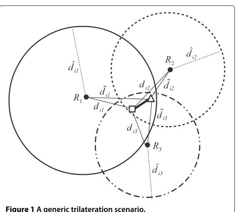
Figure 1 presents a generic triangulation scenario, including the symbolic notation used in the problem for-mulation. The scenario shows three reference nodes iden-tified byRj, j = 1, 2, 3. The circumference surrounding each reference node has radius representing the distance,
ˆ
dij, that an unknown nodeUi estimates to be from the referenceRj. The distance estimation is computed using the path loss model. The intersections of the circumfer-ences define an area where the unknown node is expected to be. The unknown node real position is denoted by ui = (uxi,uyi)and is identified by the square in the inter-section area in Figure 1. A possible candidate position for the unknown node is identified by the triangle in the same figure and is denoted byu˜i = (u˜xi,u˜ between the unknown node candidate position and each of the references is represented bydij. Additionally, the distance between a reference nodeRjand the real position of unknown nodeUiis denoted bydij.
Figure 1A generic trilateration scenario.
Ideally, consider thelog-distancemodel in (1) without the shadowing effect,
Therefore, it is straightforward to compute the estimated distance, dˆij, from the received power measurement,
ˆ From another point of view, we can think that PˆijdBm is derived from the real distance,dij, plus a shadowing error. In this case, we can derive the following relation
dij=d0·10
PdBm0 −ˆPdBmij +χ
10·η . (5) Following the derivation of [10] and combining (4) and (5) we obtain
ˆ
dij=dij·10 χ
10·η, (6) in which becomes clear that the estimated distance dˆij is affected by the shadowing in a multiplicative way, or equivalently, that the estimation error dˆij−dij
is pro-portional to the range.
In a practical localization framework, the nodes par-ticipating in the localization process should deal with power measurements. Therefore, it is convenient to refor-mulate the problem based directly on this metric. Then, assume that an unknown nodeUiis able to monitor signal transmissions from a set of reference nodes in the
neigh-borhood, denoted byR. The mean power that unknown
nodeRj ∈ R isPˆij = Pij +χ, where Pij is the power that should be received at real position of nodeUiin an ideal propagation scenario (no shadowing). Additionally, we define the mean theoretical received power at a can-didate location of nodeUi with respect to transmissions from nodes Rj ∈ R as beingPij. The proposed algo-rithm considers a cost function given by thesquared error between RSS measurements and estimated powers from references at the candidate position,
f(u˜i)=
Rj∈R
(Pˆij−Pij)2. (7)
The use of a weighting factor for the cost function that reinforces the contribution to the location from the closest references was suggested in [15], providing more precise range estimation. The proposed algorithm takes advantage from this observation and includes into the cost function a weighting factor. The weighting factor between unknown node Ui and reference node Rj reinforces the contribution from closer references and increases the location precision. The positioning algorithm evaluates as many candidate positions as required to find the one which satisfies a predefined criteria. Whenever a candi-date position for node Ui is guessed, u˜i = (u˜xi,u˜
y i), its distances to nodesRj∈Rare in turn defined as
dij=(rjx− ˜uxi)2+(ry
j − ˜u y
i)2. (8)
The estimated receiver power at the current candidate position,u˜i, can then be computed as
PdBmij =PdBm0 −10·η·log10(dij). (9)
The candidate position that minimizes f(u˜i) is the esti-mated position of the unknown node.
4 Proposed algorithm
In this section, we present the details of the proposed localization algorithm, but first we discuss the influence of ordering in the localization accuracy.
4.1 The Influence of ordering
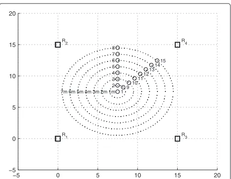
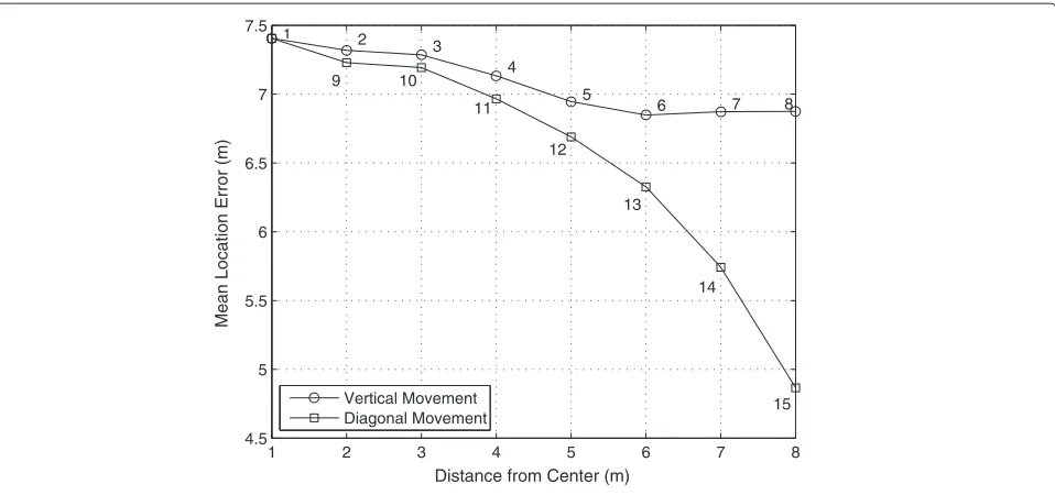
As discussed in the previous section, the localization error is proportional to the range. In order to demonstrate this effect, it was computed the mean location error for a node placed in different predefined positions, as enumerated in Figure 2. We applied the cost function defined by (7). The results for each predefined position are shown in Figure 3. The positions 1 to 8 correspond to a vertical movement of the node from the center and positions 9 to 15 corre-spond to a diagonal movement. The results clearly show that the error in range estimation is significantly reduced when the node approaches the reference R4. Therefore,
given that the real node position is determinant for the error in range estimation, it is reasonable to assume that
−5 0 5 10 15 20
Figure 2Scenario for evaluating the location error as a function of the node position.
the location ordering may affect the mean location error. Based on this assumption, we derived a metric which is a function of the node position. This metric should consider the power measurements and the correspond-ing estimated distancesdˆij, which is the only information available for the positioning algorithm. Moreover, the pro-posed algorithm first locates the node which is in the proximity of the largest number of references. Therefore, a metric is proposed to quantify the proximity of any given node to the reference nodes so that the algorithm can esti-mate which is the node closest to the largest number of references. In particular, theproximity factorof a nodeUi is computed as
whereRis the set of reference nodes in the neighborhood, which also includes the unknown nodes already localized. Computing theproximity factorfor nodes in the scenario in Figure 2, we obtain the values shown in Table 1. The first column, denoted target location sequence, presents the nodes in ascending order of location error. That is the resultant error location considering the localization of that node only. This column in Table 1 is used only as a reference, as this would be the ideal order in which the nodes should be located in case of sequential node local-ization (the node that is located with the smallest error should be located first, then it becomes a reference for the other nodes, and so on). The second and third columns, show theFproximityvalue for each nodei. A selection
1 2 3 4 5 6 7 8 4.5
5 5.5 6 6.5 7 7.5 1
2 3
4
5
6 7 8
9 10
11
12
13
14
15
Distance from Center (m)
Mean Location Error (m)
Vertical Movement Diagonal Movement
Figure 3Mean location error for different node positions.
positions associated with lower location errors should be localized first. Comparing the target sequence and the sequence obtained usingFproximity, we can verify that this
goal is not fully achieved. For example, the node in posi-tion 8 has a mean locaposi-tion error about 2 m greater than the node in position 15. We can observe in Figure 2 that when a node moves along the vertical or diagonal directions, it approaches some references and moves away from others. However, when the node is closer to a specific reference,
Table 1 Taget localization sequence and the localization sequences given by theFproximityandRproximityfactors
Target Fproximity(i) Estimated Rproximity(i) Estimated
location location location
sequence sequence sequence
15 47.6830 8 81.2738 15
14 46.6297 15 63.4042 14
13 46.1839 7 51.9312 13
12 45.5853 14 43.9526 12
8 44.9661 6 39.1365 8
7 44.6653 13 38.2657 7
6 44.0120 5 38.0920 11
5 43.8848 12 36.8669 6
11 43.2998 4 35.1000 5
4 43.2586 11 33.6129 10
10 42.8085 3 33.1326 4
9 42.8002 10 31.1058 3
3 42.5210 2 30.0848 9
2 42.5205 9 29.1206 2
1 42.4264 1 27.2395 1
its mean location error achieves a lower value. Based on this observation, a new metric was empirically derived, calledproximity relation, which is a function ofFproximity
and the lowest distancedˆij estimated (measured) by the unknown nodeUito a referenceRjor an already localized node. The set of unknown nodes already localized will be denoted byL. Theproximity relationis defined as
Rproximity(i)=
Fproximity(i)·α+γ
min(dˆij)
, ∀j∈ {R∪L}.
(11)
where
α=
1.15, for 1≤j≤m
1, forj>m. (12)
Based on simulation experiments, we identified that the distance estimates between two unknown nodes not yet localized can be used to improve the sequence ordering used by the localization algorithm. This is done by adding toFproximitythe constant parameterγ =(n−|L|)·max(D),
wherenis the number of unknown nodes,|L|is the car-dinality ofL, andD = [dˆij] is the matrix of estimated distances. The scaling factorαhas the objective to locate unknown nodes that are closer to a great number of ref-erence nodes. Therefore, if there are two unknown nodes with the same value of Rproximity(i), the one that has a
indicated in Figure 2 are also presented in Table 1. Note that theestimated location sequence obtained based on Rproximityis very close to thetargetlocation sequence.
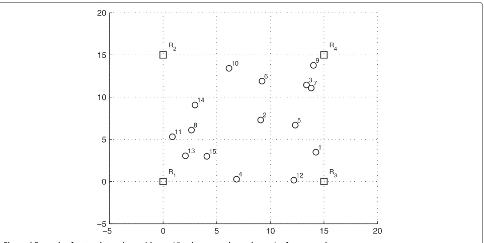
As another example, consider the network topol-ogy of Figure 4. By applying the Rproximity factor to
determine the localization ordering of the unknown nodes, they will be located in the following order:
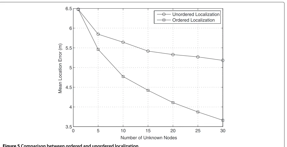
{9, 3, 7, 12, 13, 15, 11, 8, 14, 1, 4, 5, 2, 6, 10}. Each located node that becomes a reference node affects the metric for the next nodes. This means that unknown nodes closer to already located nodes will be localized first. Figure 5 presents a comparison between the performance of the location algorithm with and without node ordering, as a function of the number of unknown nodes in the network. It should be pointed out that the location error can be sig-nificantly reduced when the number of unknown nodes increases, which we consider to be a quite interesting feature.
4.2 Algorithm
The proposed algorithm locates nodes individually, fol-lowing the sequence ordering obtained using theRproximity
factor, where the node with the highestRproximityfactor is
located first. The pseudocode is presented in Algorithm 1. The set of reference nodes,R, have known coordinates, rj. These nodes collect the power measurements from unknown neighbor nodes to form matrix Pˆ. The refer-ence power P0dBm and the pathloss exponentη are pre-defined parameters. Based on the power measurements, the Rproximity factor is computed for all unknown nodes.
Then, the iterative localization procedure is started, where
the unknown nodes are localized in the order based on the Rproximity factor. The coordinates are estimated by
minimizing the cost functionf(u˜k). The localized node becomes part of the reference set for the next iteration of the algorithm.
Algorithm 1:
1.1 Input Parameters:
1.2 Pˆ =[PˆdBmij ] : Matrix of power measurements 1.3 rj=(rxj,r
y
j),∀Rj∈R: Reference nodes coordinates
1.4 PdBm0 : Reference power at a reference distanced0
1.5 η: Path loss exponent 1.6 ComputeRproximity(i),∀Ui∈U
1.7 Define the empty set,L= {∅} 1.8 While|L|<|U|
1.9 Select unknown nodeUk ∈U, where
k=arg max i
Rproximity(i)
1.10 Select an initial candidate position for
unknown nodeUk,u˜k=(u˜xk,u˜ y k)
1.11 min
˜
uk f(u˜k)=
j∈{RL}
βkj·(Pˆkj−Pkj)2
1.12 Setuˆk= ˜ukand update setL= {LUk}
1.13 end
Note that in the proposed algorithm, we include a scale factorβijfor the cost function terms (please compare step (1.11) of Algorithm 1 and (7)). The inclusion of the scale
−5 0 5 10 15 20
−5 0 5 10 15 20
R 1 R
2
R 3 R
4
1 2
3
4
5 6
7
8
9 10
11
12 13
14
15
0 5 10 15 20 25 30 3.5
4 4.5 5 5.5 6 6.5
Number of Unknown Nodes
Mean Location Error (m)
Unordered Localization Ordered Localization
Figure 5Comparison between ordered and unordered localization.
factor is based on the fact that the error in the estima-tion of relative distancedˆijincreases for greater distances betweeni and j. The scaling factor β uses the relation betweenFproximity(i)in (10) and the estimated distancedij between unknown nodeiand reference nodejas a way to attribute a higher scale factor to an unknown node closest to the reference. The parameterβkjis computed as
βkj=ρ·log
Fproximity(i) dkj
(13)
whereρis a constant which benefits the proximity of an unknown node to any reference and whose optimal value obtained through extensive simulations isa
ρ=
2.7, for 1≤j≤m
1, forj>m. (14)
In Figure 6, we present a comparison between the per-formance of the proposed algorithm with and without the proposed scale factorβijin the cost function, considering the same scenario with four reference nodes presented in Figure 4. It is clear that the inclusion of the scaling factor is beneficial in terms of performance.
Moreover, in our implementation, we use of the Nelder-Mead nonlinear optimization numerical method [9] for minimizing the weighted cost function, therefore without requiring the derivative of the cost-function, as is the case of MLE methods based on the conjugate gradient [10].
4.3 Initial candidate position problem
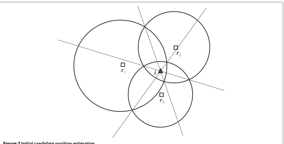
For practical implementations of localization algorithms, the best strategy to select the initial candidate positions for unknown nodes is to apply the method proposed in [19], which selects the initial candidate position based on estimated distances from reference nodes. Consider the scenario shown in Figure 7, with reference nodesr1, r2,
andr3. The circumferences surrounding each reference
node represent the estimated distances for unknown node kand are defined as
(u˜xk−rx1)2+(u˜yk−ry1)2=d1k, (15)
(u˜xk−rx2)2+(u˜yk−ry2)2=d2k, (16)
(u˜xk−rx3)2+(u˜yk−ry3)2=d3k. (17)
By combining (15) and (16), we obtain
(rx2−rx1)· ˜ukx+(ry2−ry1)· ˜uky=d21k−d22k+(rx2)2−(rx1)2
+(r2y)2−(ry1)2/2
(18)
which is the equation that represents the straight line defined by the two intersection points of circles defined by (15) and (16). Similarly, by combining (15) with (17) and (16) with (17), we obtain the other two line equations:
(rx3−r1x)· ˜ukx+(ry3−r1y)· ˜uky= d12k−d32k+(r3x)2−(rx1)2
+(ry3)2−(r1y)2/2, (19)
(rx3−r2x)· ˜ukx+(ry3−r2y)· ˜uky= d22k−d32k+(r3x)2−(rx2)2
+(ry3)2−(r2y)2
0 5 10 15 20 25 30 3
3.5 4 4.5 5 5.5 6 6.5
Number of Unknown Nodes
Mean Location Error (m)
without with Beta
Figure 6Effect of the scaling factors in the location error.
The intersection of these three straight lines defines the initial candidate position of unknown nodekfor the local-ization algorithm, as marked by the triangle in Figure 7. In a specific scenario, where the three references are aligned, the lines are parallel. In such case, the initial candidate position is defined as the mean computed among the coordinates defined by the intersection of the line defined by the references with the parallel lines [19].
5 Practical results
The design of the proposed algorithm is heavily based on extensive computer simulations. Therefore, in order to evaluate the effectiveness of our approach, we tested the proposed localization algorithm in a real wireless network scenario implemented in an outdoor environ-ment, as shown in Figure 8. The scenario consists of one unknown node designated byiand three reference nodes
Figure 8Real wireless network setup implemented in an outdoor environment.
denoted by Rj, j = 1, 2, 3. The wireless nodes consist of mobile devices equipped with IEEE802.11b interfaces, operating in channel number 4 (carrier frequency 2,417 MHz). This channel was selected because it was the free available frequency band without co-channel and adjacent channel interferences at the moment.
The path loss exponent required by the algorithm,η, was determined from RSS measurements in a range dis-tance from 10 to 100 m, in steps of 10 m. At each disdis-tance, d, a set of 1,000 RSS samples were collected to determine the average values in the downlink and uplink channels. These average values are plotted in Figure 9. The aver-age noise power in the wireless interfaces was measured as−100 dBm. The estimated value ofη, using the mini-mum mean squared error (MMSE) method, was obtained asη = 2.4 for downlink andη = 2.2 for uplink. In the positioning algorithm, we used the mean value,η=2.3. In the practical survey, five scenarios were considered. The configuration parameters and measured powers of each scenario are summarized in Table 2. The localization algo-rithm considers the average power values,Pj, measured
100 101 102
0 20 40 60 80
Distance (m)
RSS(dB) − Downlink
2.4
100 101 102
0 20 40 60 80
Distance (m)
RSS(dB) − Uplink
2.2
Figure 9Estimated path loss exponent.
Table 2 Power measurements in each scenario
Scenariodi1 di2 di3 P1 σP21 P2 σ 2
P2 P3 σ 2 P3
(m) (m) (m) (dBm) (dBm2) (dBm) (dBm2) (dBm) (dBm2)
A 5 5 5 –37.84 0.80 –38.04 0.66 –41.83 1.32
B 10 10 10 –45.38 0.57 –45.57 0.63 –50.31 1.32
C 20 20 20 –50.93 1.48 –50.65 0.49 –54.70 1.16
D 50 50 50 –54.86 1.04 –55.47 0.64 –57.76 1.54
E 20 10 50 –51.01 1.69 –44.42 0.78 –56.03 0.62
at each reference nodej, as shown in Table 2, which also shows the variance of the collected power samples,σP2
j. In order to apply the proposed localization algorithm, it is necessary to first determine the received reference power,P0, at a reference distance,d0, from the
transmit-ter. The received signal power at reference distanced0is
computed using
P0dBm=PtdBm+GdBit +GrdBi−2·LdBc −LdB0 , (21)
whereLdB0 is the free space path loss for a reference
dis-tance d0 = 1 m. The parameters used in (21) were
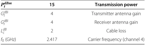
obtained from equipment specifications and are pre-sented in Table 3.
In order to evaluate the performance of the proposed algorithm, we compared it with the classical MLE [10] which is based on the conjugated gradient optimization methodb. The practical results in terms of location error are presented in Figure 10 using the weighted cost func-tion with parameter β as defined by (13). The results show that the use of a weighted cost function can lead to considerable reductions in localization errors in all prac-tical network scenarios. For scenario E, this reduction may reach approximately 30%. Even for scenarios A and B, a low but significant reduction around 3% is achieved. When the β scale factor is applied to the cost function, the higher reported RSS receives a higher weight because they correspond to more precise measurements obtained from reference nodes closer to the unknown node. This explains the best result obtained for scenario E, where the distances from the three reference nodes to the unknown node are different.
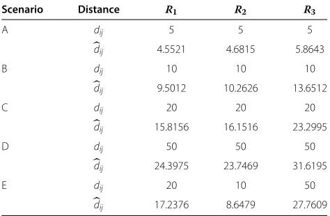
Some additional insights can be obtained analyzing the data shown in Table 4 and Figure 10. For each sce-nario, this table presents the real distancesdijamong the
Table 3 Wireless interface parameters
PtdBm 15 Transmission power
GdBi
t 4 Transmitter antenna gain
GdBi
r 4 Receiver antenna gain
LdB
c 2 Cable loss
A B C D E
Figure 10Location error and error reduction obtained with the proposed algorithm for the real world scenarios.
unknown node and the reference nodes, as well as the esti-mated distancesdij. For scenarios A, B, and C, the mean reported RSS values caused a positive error in distance estimation, mainly for the values measured with respect to referenceR3. It means that the unknown node is sensed
to be farther away from this reference than it really is. The more distant are nodes i andj, the lower is the weight of its RSS value in the cost function and therefore the erroneous RSS measures have less influence in the opti-mization. This can lead to error reductions of up to 12% in these scenarios with respect to the MLE algorithm, as seen in Figure 10. Scenario D presents large values of neg-ative errors in distance estimation, so the unknown node seems to be closer to reference nodes than it really is. The relative distance estimation toR3was more accurate with
respect to real distancedi3=50 m. By observing Figure 8,
we can verify that node i is positioned exactly between R1 and R2. Therefore, even if the RSS values between
Table 4 Actual and estimated distances
Scenario Distance R1 R2 R3
A dij 5 5 5
dij 4.5521 4.6815 5.8643
B dij 10 10 10
dij 9.5012 10.2626 13.6512
C dij 20 20 20
dij 15.8156 16.1516 23.2995
D dij 50 50 50
dij 24.3975 23.7469 31.6195
E dij 20 10 50
dij 17.2376 8.6479 27.7609
nodeiand references R1 andR2 are inaccurate, there is
a tendency of the algorithm to optimize the location ofi equidistant toR1andR2since then the average reported
powers to these references have similar values, as was the case. The weighting factorβreduces the localization error even more when it attributes higher weights to RSS values reported fromR1andR2, because referenceR3reported a
lower RSS value, even though more precise.
6 Conclusions
In this paper, we present a new localization strategy based on RSS measurements. The algorithm is centralized and iterative: centralized because a node must accumulate the RSS measurements and run the location algorithm for all the other nodes; iterative because each node is localized one at a time and once located it becomes a reference to the location of other unknown nodes in the next itera-tions. The Nelder-Mead nonlinear optimization numeri-cal method is employed to find the candidate coordinates for the unknown node, by minimizing the cost function. It is shown that the proposed algorithm can achieve bet-ter practical position estimates than the classical MLE strategy that employs gradient-search-based methods.
Endnotes
aThere are two constants that are used in our proposed
algorithm and that were numerically obtained (αandρ). These values were obtained after several tests
considering up ton=30 unknown nodes randomly located within an area of 15×15 m2(the node positions are random and follow a uniform distribution). For each number of unknown nodes, an ensemble of topologies were generated and several values ofαandρwere tested. The impact ofρin the performance of the proposed algorithm is larger than the impact ofα.
bAmong existing classical cooperative localization
techniques for wireless networks, the MLE is theoretically the best in the sense that it asymptotically achieves the Cramer-Rao bound (CRB). However, the gradient based iterative algorithms that are commonly used to achieve MLE positions are quite sensitive to the initial values and cannot achieve the theoretical optimal performance [14]. In this case the optimum solution is the minimum mean square error (MMSE) algorithm, which requires the prior distribution on the location of the nodes.
Competing interests
The authors declare that they have no competing interests.
Acknowledgements
This work was partially supported by CAPES and CNPq (Brazil).
Author details
Received: 5 June 2013 Accepted: 7 November 2013 Published: 5 December 2013
References
1. P Gupta, PR Kumar, The capacity of wireless networks. IEEE Trans. Inf. Theory46(2), 388–404 (2000)
2. K-F Kao, I-E Liao, J-S Lyu, An indoor location-based service using access points as signal strength data collectors, in2010 International Conference On Indoor Positioning and Indoor Navigation (IPIN). Campus Science City, ETH Zurich, 15-17 Sept 2010
3. I Sabek, M Youssef, Multi-entity device-free wlan localization, in2012 IEEE Global Communications Conference (GLOBECOM). Anaheim, 3-7 Dec 2012 4. P Riedl, R Mayrhofer, Towards a practical, scalable self-localization system
for android phones based on wlan fingerprinting, in2012 32nd International Conference On Distributed Computing Systems Workshops (ICDCSW). Macau, 18-21 June 2012
5. D Felix, M McGuire, Received signal strength calibration for handset localization in wlan, in2012 IEEE International Conference On Communications (ICC). Ottawa, 10-15 June 2012
6. V Bhargava, ML Sichitiu, Physical authentication through localization in wireless local area networks, inGLOBECOM ’05 IEEE Global
Telecommunications Conference. vol. 5 (IEEE, Picastaway, 2005) 7. N Patwari, JN Ash, S Kyperountas, IAO Hero, RL Moses, NS Correal,
Locating the nodes: cooperative localization in wireless sensor networks. IEEE Signal Processing Magazine22(4), 54–69 (2005)
8. C-D Wann, H-C Chin, Hybrid toa/rssi wireless location with unconstrained nonlinear optimization for indoor uwb channels, inIEEE Wireless Communications and Networking Conference (WCNC 2007). Hong Kong, 11-15 March 2007
9. JA Nelder, R Mead, A simplex method for function minimization. Comput. J.7(4), 308–313 (1965)
10. N Patwari, RJ O’Dea, Y Wang, Relative location in wireless networks, inIEEE VTS 53rd, Vehicular Technology Conference, 2001. VTC 2001 Spring. vol. 2, (IEEE, Piscataway, 2001)
11. H Wymeersch, J Lien, MZ Win, Cooperative localization in wireless networks. Proc. IEEE.97(2), 427–450 (2009)
12. C Pedersen, T Pedersen, BH Fleury, A variational message passing algorithm for sensor self-localization in wireless networks, in2011 IEEE International Symposium On Information Theory Proceedings (ISIT). St. Petersburg, 31 July–5 Aug 2011
13. V Savic, S Zazo, Cooperative localization in mobile networks using nonparametric variants of belief propagation. Ad Hoc Netw.11(1), 138–150 (2013)
14. S Xi, MD Zoltowski, A practical complete mle cooperative localization solution, in2010 IEEE International Conference On Acoustics Speech and Signal Processing (ICASSP). Dallas, 14–19 March 2010
15. A Savvides, C.-c Han, MB Strivastava,Dynamic Fine-Grained Localization in Ad-Hoc Networks of Sensors, inProceedings of the 7th annual international conference on Mobile computing and networking, (MobiCom 2001). (ACM, New York, 2001), pp. 166-179
16. S Gezici, A survey on wireless position estimation. Wireless Personal Commun.44(3), 263–282 (2008)
17. T Rappaport,Wireless Communications: Principles and Practice,2nd edn. (Prentice Hall, Upper Saddle River, 2001)
18. A Goldsmith,Wireless Communications(Cambridge University Press, New York, 2005)
19. H-L Song, Automatic vehicle location in cellular communications systems. Vehicular Technol., IEEE Trans.43(4), 902–908 (1994)
doi:10.1186/1687-1499-2013-276
Cite this article as:Trevisanet al.:A simple iterative positioning algorithm for client node localization in WLANs.EURASIP Journal on Wireless Communi-cations and Networking20132013:276.
Submit your manuscript to a
journal and benefi t from:
7Convenient online submission
7Rigorous peer review
7Immediate publication on acceptance
7Open access: articles freely available online
7High visibility within the fi eld
7Retaining the copyright to your article