R E S E A R C H
Open Access
Distributed resource allocation for MISO
downlink systems via the alternating direction
method of multipliers
Satya Krishna Joshi
*, Marian Codreanu and Matti Latva-aho
Abstract
We provide distributed algorithms for the radio resource allocation problem in multicell downlink multi-input single-output systems. Specifically, the problems of (1) minimizing total transmit power subject to
signal-to-interference-plus-noise ratio (SINR) constraints of each user and (2) SINR balancing subject to total transmit power constraints are considered. We propose a consensus-based distributed algorithm and the fast solution method via alternating the direction method of multipliers. First, we derive a distributed algorithm for minimization of total transmit power. Then, in conjunction with the bracketing method, a distributed algorithm for SINR balancing is derived. Numerical results show that the proposed distributed algorithms achieve the optimal centralized solution.
Keywords: Distributed optimization; Multicell networks; Minimum power beamforming;
Signal-to-interference-plus-noise ratio (SINR) balancing; Alternating direction method of multipliers (ADMM); Dual decomposition; Second-order cone program (SOCP)
1 Introduction
We provide distributed algorithms for the problem of resource allocation for multicell downlink systems with linear precoding. The base stations (BSs) are assumed to have multiple antennas while all the users are equipped with single antenna. Full channel state information is assumed to be available at both the BSs and the users, and all the users share the same frequency bandwidth. Under this setting, we consider the following two optimization problems: P1 - minimization of the total transmission power subject to minimum signal-to-interference-plus-noise ratio (SINR) constraints of each user, and P2 - SINR balancing subject to total transmit power constraint of BSs.
Several centralized algorithms for problems P1 and P2 have been proposed in the literature. See, e.g., [1-6] for problem P1 and [7-10] for problem P2. Unfortunately, the centralized method is not practical for the resource allocation due to high overhead required for collecting all channel state information at the central processing
*Correspondence: sjoshi@ee.oulu.fi
Centre for Wireless Communications, University of Oulu, P.O. Box 4500, Oulu FI-90014, Finland
unit. Therefore, to share the workload of the central con-troller and to overcome impelling backhaul overhead, the distributed algorithm is desirable in practice.
Distributed methods for problem P1 for multiple-input and single-output (MISO) multicell wireless systems have been proposed in [11-15]. The algorithm in [11] is based on uplink-downlink duality, where the minimum power downlink beamformers designing problem is solved using a dual uplink problem. The algorithm in [11] is a multi-cell generalization of the algorithm proposed in [16] for the single-cell case. In [12] dual decomposition method is adopted, and the algorithm in [13] is based on primal decomposition. Both in primal and dual decomposition methods [17], the master problem is solved using an iter-ative method such as the subgradient method [18]. Even though problem P1 is a convex problem and can be eas-ily solved via primal or dual decomposition (see, [12,13]), the convergence speed of those algorithms are slow and highly sensitive on the subgradient step size [18]. A game theoretic approach is considered in [14].
Problem P2 is a quasiconvex problem [16]. Thus, the centralized method based on bisection search [19] is com-monly used, e.g., [10,16]. Combining the bisection search and the uplink-downlink SINR duality, a distributed
algorithm is proposed in [20]. The algorithm in [20] is a hierarchical iterative algorithm which consists of outer and inner iterations, where the bisection search is car-ried out in the outer iteration and uplink-downlink SINR duality is used for the inner iteration.
The alternating direction method of multipliers (ADMM) is a simple but powerful algorithm that is well suited to distributed convex optimization. ADMM com-bines the benefits of dual decomposition and augmented Lagrangian methods [21]. Hence, ADMM is numerically stable than dual decomposition and hence suitable for many practical optimization problem [21]. Due to supe-rior stability properties and decomposability, ADMM has been applied to a wide rage of applications, such as com-pressed sensing [22], image restoration [23], signal pro-cessing [15,24,25], etc.; see [21] for the recent survey. In many applications, the ADMM method has been observed to converge fast [21,26,27]; and when the objective func-tion is strongly convex and Lipschitz continuous, ADMM can even guarantee the liner rate of convergence [28,29].
The main contribution of the paper is to propose consensus-based distributed algorithms for problems P1 and P2, and the fast solution method via ADMM [21]. The ADMM turns the original problem into a series of itera-tive steps, namely,local variable update,global variable update, anddual variableupdate [21]. The local variable and dual variable updates are carried out independently in parallel by all BSs, while the global variable update is car-ried out by BS coordination. In this paper, we first derive distributed algorithm for problem P1. Then, we extend the formulation of problem P1 to derive the distributed algorithm for problem P2. In particular, we recast the problem into a more tractable form and combine bracket-ing method (e.g., golden ratio search) [30,31] with ADMM to derive the distributed algorithm for problem P2.
Recently, for problem P1, by considering the uncer-tainty in the channel measurements, an algorithm based on ADMM has been proposed in [15]. In our paper, we consider perfect channel state information (CSI) and use the consensus technique to solve the problem. Then, we apply ADMM to derive the distributed algorithm. The consensus technique can be easily decomposed into a set of subproblems suitable for distributed implementation [21,24]. Hence, the algorithm formulation in this paper is more intuitive than that provided in [15]. It is worth noting that this paper extends our recent work [32] to SINR balancing problem (i.e., problem P2). In addition, for problem P1, we show that the proposed distributed algorithm converges to the optimal centralized solution. Moreover, for problem P1, we also provide a method to find the ADMM penalty parameter that leads faster convergence of the algorithm.
Note that problem P2 is a quasiconvex problem. To the best of our knowledge there is no convergence theory to
the ADMM method for a quasiconvex problem. How-ever, if each step of the ADMM iteration is tractable, the ADMM algorithm can still be used to derive (pos-sibly suboptimal) distributed methods for problem P2 [21, Chapter 9]. Though these methods are not provably optimal, our numerical results show that the proposed algorithm converged to the optimal solution in all simulated cases.
The remainder of this paper is organized as follows. The considered MISO system model and problem formula-tion are described in Secformula-tion 2. The distributed algorithm for sum power minimization (P1) is derived in Section 3. Next, in Section 4, we derive the distributed algorithm for SINR balancing problem (P2). The numerical results are presented in Section 5, and Section 6 concludes our paper. Notations: All boldface lower case and upper case letters represent vectors and matrices, respectively, and calligra-phy letters represent sets. The notationCTdenotes the set of complexT-vectors,|x|denotes the absolute value of the scalarx,x2denotes the Euclidean norm of the vectorx,
Idenotes the identity matrix, andCN(m,C)denotes the complex circular symmetric Gaussian vector distribution with meanmand covariance matrixC. The superscripts
(·)H and (·) are used to denote a Hermitian transpose
of a matrix and a solution of an optimization problem, respectively.
2 System model and problem formulation
A multicell MISO downlink system, with N BSs each equipped withTtransmit antennas, is considered. The set of all BSs is denoted byN, and we label them with the integer valuesn = 1,. . .,N. Thetransmission regionof each BS is modeled as a disc with radiusRBScentered at the location of the BS. Single data stream is transmitted for each user. We denote the set of all data streams in the system byL, and we label them with the integer values l=1,. . .,L. The transmitter node (i.e., the BS) oflth data stream is denoted by tran(l), and the receiver node oflth data stream is denoted by rec(l). We haveL= ∪n∈NL(n),
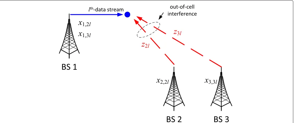
whereL(n)denotes the set of data streams transmitted by nth BS. Note that the intended users of the data streams transmitted by each BS are necessarily located inside the transmission region of the BS (see Figure 1).
The antenna signal vector transmitted by nth BS is given by
xn=
l∈L(n)
dlml, (1)
−10 −5 0 5 10 15 20 25
The signal received at rec(l)can be expressed as
yl=dlhHllml+
j∈L(tran(l)),j=l djhHjlmj
(intra-cell interference)
+
n∈N\{tran(l)}
j∈L(n)
djhHjlmj+nl,
(out-of-cell interference)
(2)
wherehHjl ∈ C1×T is the channel matrix between tran(j)
and rec(l), andnlis circular symmetric complex gaussian noise with varianceσl2. Note that the second right hand term in (2) represents the intra-cell interference and the third right hand term represents the out-of-cell interfer-ence. The received SINR of lth data stream is given by
l= |h out-of-cell interference fromnth BS to rec(l).
The out-of-cell interference term in (3) (i.e.,
n∈N\{tran(l)}z2nl) prevents resource allocation on an intra-cell basis and demands BS coopera-tion/coordination. To avoid unnecessary coordination between far apart-located BSs, we make the following assumption: transmission from nth BS interfere the lth data stream (transmitted by BSb=n) only if the distance between nth BS and rec(l) is smaller than a threshold Rinta. The disc with radiusRintcentered at the location of any BS is referred to as theinterference regionof the BS (see Figure 1). Thus, ifnth BS located at a distance larger thanRintto rec(l), the associatedznl components are set
to zerob. Based on the assumption above, we can express
las fering BSs that are located at a distance less thanRintto rec(l). For example, in Figure 1a, we haveNint(2) = {2}, Nint(8) = {1}, andNint(l) = ∅for alll ∈ {1, 3, 4, 5, 6, 7}. Moreover, it is useful to define the set Lint of all data streams that are subject to the out-of-cell interference, i.e.,
Lint = {l|l ∈ L,Nint(l) = ∅}. For example, in Figure 1a, we haveLint= {2, 8}.
The total transmitted power of the multicell downlink system can be expressed as
P=
n∈N
l∈L(n) ml22.
Assuming that the SINR l is subject to the constraint
l ≥ γlfor each userl ∈ L, the problem of minimizing the total transmitted power (i.e., P1) can be expressed as
P1 : minimize
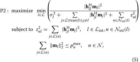
fairness among the users is by maximizing the minimum SINR (i.e., P2) [16], which can be formulated as
P2 : maximize min l∈L
Finally, to improve the readability of the paper, we sum-marize a list of sets used in this paper in Table 1.
3 Sum power minimization
In this section, we derive a distributed algorithm for prob-lem (4), i.e., P1. First, we equivalently reformulate the original problem (4) in a form ofglobal consensus prob-lem. Then, we derive the proposed distributed algorithm based on ADMM [21].
3.1 An equivalent reformulation: sum power
minimization
We start by reformulating sum power minimization prob-lem (4) as
Table 1 Summary of a list of sets
Set Description
N Set of all BSs
L Set of all data streams
L(n) Set of data streams transmitted bynth BS Nint(l) Set of out-of-cell BSs interfering tolth data stream Lint Set of all data streams that are subject to the out-of-cell
interference
Iint(n) Set of links for which BSnacts as the out-of-cell interferer Lint(n) Set of links in BSnthat are affected by the out-of-cell
interference
where the variables are {ml}l∈L and {znl}l∈Lint,n∈Nint(l).
Problems (4) and (6) are equivalent as it can be easily shown (e.g., by contradiction) that the second inequality holds with equality at the optimal point.
Recall that z2nl in problem (6) represents power of the out-of-cell interference caused by nth BS at rec(l), and hence, variable znl couples exactly two BSs (i.e., BS n and BS tran(l)). We use consensus technique to distribute problem (6) over the BSs. The method consist of introduc-ing local copies of the couplintroduc-ing variablesznlfor alll∈Lint, n∈Nint(l)at each BS (see Figure 2).
Let us definexk,nlas the local copy ofznlat BSk. Thus for eachznl, we make two local copies, i.e.,xn,nlat BSnand xtran(l),nl at BS tran(l). Then, problem (6) can be written equivalently in aglobal consensusform as
minimize straints of (7), we have replaced znl by the local copy xn,nl. The last set of equality constraints of (7) are called consistency constraints, and they enforce the local copies {xk,nl}k∈{n,tran(l)} to be equal to the corresponding global
variableznl.
Problem (7) is not a convex problem. However, by fol-lowing the approach of [16, Section IV-B], problem (7) can be equivalently cast in the form of convex problem. To do this, let us define the matrixMn=[ml]l∈L(n)obtained by
concatenating the column vectorsml. Then, by following the approach of [16, Section IV-B], problem (7) can be equivalently reformulated in the form of convex problem as
Figure 2Illustration of BS coupling, and introducing local copies to decouple a problem.BS 2 and BS 3 are coupled with BS 1 due to coupling variablesz2landz3l, respectively. To distribute the problem, local copyx1,2lofz2lat BS 1 and local copyx2,2lofz2lat BS 2 are introduced. Similarly, local copyx1,3lofz3lat BS 1 and local copyx3,3lofz3lat BS 3 are introduced.
with variables {Mn}n∈N, {xk,nl}k∈{n,tran(l)},l∈Lint,n∈Nint(l),
and{znl}l∈Lint,n∈Nint(l), where vector x˜l = {xn,bl}b∈Nint(l),
the matrixhjlin the second set of constraints denotes the channel from BSnto linkl(i.e., the indexjin the second set of constraints denotes an arbitrary link inL(n)), and the notation SOC denotes the generalized inequalities with respect to the second-order cone [16,19].
In problem (8), the objective function and the first set of inequality constraints are separable in n ∈ N (one for each BS). Also, it can be easily shown that the sec-ond set of inequality constraints of (8) are separable in n∈N. To do this, let us denoteIint(n)the set of links for which BSnacts as an out-of-cell interferer, i.e.,Iint(n)= {l|l ∈ Lint,n ∈ Nint(l)}. Then, by noting that the sets {(n,l)|l∈Lint,n∈Nint(l)}, and{(n,l)|n∈N,l∈Iint(n)} are identical, the second set of inequality constraints of (8) can be written as
xn,nl
MnHhjl
SOC0, n∈N,l∈Iint(n), (9)
which is separable inn ∈ N. Observe that without the consistency constraints, problem (8) can now be easily decoupled intoNsubproblems, one for each BS.
We next express problem (8) more compactly. To do this, we first express the consistency constraints of prob-lem (8) more compactly by using vector notations, which denote a collection of the local and global variables associ-ated with BSn. By using the equivalence between the sets {(n,l)|l∈Lint,n∈Nint(l)}and{(n,l)|n∈N,l∈Iint(n)}, let us express the consistency constraints of problem (8) as
xn,nl =znl, n∈N,l∈Iint(n) xtran(l),nl =znl, l∈Lint,n∈Nint(l).
(10)
In the first set of equalities of (10), {xn,nl}l∈Iint(n) is a
set of local variables that are associated with BSn. Simi-larly, to find a set of local variables that are associated with BSnin the second set of equalities of (10), let us define
Lint(n) the set of links in BS n that are affected by the out-of-cell interference, i.e.,Lint(n)= {l|l∈Lint∩L(n)}. Then, by noting that the setLint = ∪n∈NLint(n), we can rewrite (10) as
xn,nl=znl, n∈N,l∈Iint(n)
xtran(l),bl=zbl, n∈N,l∈Lint(n),b∈Nint(l). (11)
Clearly, in the second set of equalities of (11)e, {xtran(l),bl}l∈Lint(n),b∈Nint(l)is a set of local variables that are
associated with BSn.
We now denote (11) compactly using vector notation. Let us define vectorsxnandznasf
xn= {{xn,nl}l∈Iint(n),{xtran(l),bl}l∈Lint(n),b∈Nint(l)}
zn= {{znl}l∈Iint(n),{zbl}l∈Lint(n),b∈Nint(l)}.
(12)
Then, (11) can be compactly written as
xn=zn, n∈N. (13)
Furthermore, for the sake of brevity, let us define the
and the following function
fn(Mn,xn)=
Then by using notations (13), (14), and (15), consensus problem (8) can be written compactly as
minimize
3.2 Distributed algorithm via ADMM: sum power
minimization
In this section, we derive distributed algorithm for prob-lem (16). The proposed algorithm is based on ADMM [21]. We start by writing theaugmented Lagrangian[33] for problem (16) as
Lρ({Mn,xn}n∈N,{zn}n∈N,{un}n∈N)
the equality constraints of (16), andρ > 0 is a penalty parameterthat adds the quadratic penalty to the standard LagrangianL0for the violation of the equality constraints of problem (16).
Each iteration of ADMM algorithm consists of the fol-lowing three steps [21]
Min+1,xin+1=argmin
where superscript i is the iteration counter. Steps (18) and (20) are completely decentralized, and hence, they can be carried out independently in parallel in each BS. Note that each component ofzncouples two local variables that
are associated with the adjacent BSs (see, consistency con-straint of problem (8))h. Thus, step (19) requires to gather the updated local variables(Min+1,xin+1)and the dual vari-ablesuinfrom allNBSs. In the sequel, we first explain in detail to solve the ADMM steps in (18) and (19). Then, we summarize the proposed ADMM based distributed algorithm.
The local variable update(Min+1,xin+1)in (18) is a solu-tion of the following optimizasolu-tion problem
minimize fn(Mn,xn)+uiTn (xn−zin)+ is a scaled dual variable). Then by using notations (14) and (15), problem (21) can be equivalently expressed as
minimize the second set of constraints denotes the channel from BS nto linkl(i.e., the indexjin the third set of constraints denotes an arbitrary link inL(n)), and the notationSOC denotes the generalized inequalities with respect to the second-order cone [16,19]. Note that in the objective function of (22)i, we have dropped a constant termρ2vin22
since it does not effect the solution of the problem. Moreover, by writing problem (22) in the epigraph form, and then following the approach of [16, Section IV-B], problem (22) can be equivalently reformulated in the form of second-order cone program (SOCP) as
with variablest,Mn, andxn. Let us denotet,Mn, andxn
the solutions of problem (23), then the updateMin+1=Mn
andxin+1=xn.
Now, we turn to the second step of ADMM algorithm and provide a solution for the global variable update (19). The update{z}in+1}n∈N is a solution of the following
opti-mization problem
minimize n∈N
uiTn (xin+1−zn)+
ρ
2x i+1 n −zn22
,
(24)
with variable {zn}n∈N. By using the notations in (12),
and further noting equalities (13) and the equality con-straints of problem (8) are equivalent, problem (24) in the components ofxn,zn, anduncan be expressed as
minimize l∈Lint
n∈Nint(l)
k∈{n,tran(l)} ×uik,nl(xki+,nl1−znl)+
ρ
2(x i+1 k,nl−znl)2
,
(25)
with variable {znl}l∈Lint,n∈Nint(l), where
{uk,nl}k∈{n,tran(l)},l∈Lint,n∈Nint(l) are the dual variables
associated with the equality constraints of problem (7)j. Problem (25) decouples across znl, since the objec-tive function is separable in znl for all l ∈ Lint,n ∈ Nint(l). Moreover, the objective function of problem (25) is quadratic inznl. Hence, by setting the gradient of (25) with respect toznlequal to zero, we can get the solution z
nlwhich can be expressed as
znl=
xni+,nl1+xtrani+1(l),nl+ 1
ρ(u
i
n,nl+uitran(l),nl)
!
2,
(26)
for alll ∈ Lint,n ∈ Nint(l). Therefore, the updateznli+1 = znl for alll ∈ Lint,n ∈ Nint(l). Moreover, by substituting zinl+1in (20)k, we can show that the sum of the dual vari-ablesuin,nl +uitran(l),nl is equal to zero. Thus, the update zinl+1further simplifies to
zinl+1=
xni+,nl1+xtrani+1(l),nl
"
2, (27)
for alll ∈ Lint,n ∈ Nint(l). Hence, the global variable updatezinl+1is simply the average of its local copiesxin+,nl1 andxitran+1(l),nl.
Finally, we summarize the proposed ADMM-based dis-tributed algorithm for sum power minimization prob-lem (8) in Algorithm 1.
Algorithm 1 Proposed ADMM-based distributed
algorithm for sum power minimization
1 Initialization: given SINRs target{γl}l∈L and penalty ρ >0. Seti=0,{u0n}n∈N =0, and{z0n}n∈N =0.
2 BSn=1. . .Nupdate local variables(Mni+1,xin+1). 3 BSnand BS tran(l)exchange their local copiesxin+,nl1 andxitran+1(l),nlfor alll∈Lint,n∈Nint(l).
4 BSn=1. . .Nupdate global variablezin+1. 5 BSn=1. . .Nupdate dual variableuin+1.
6 If stopping criteria is satisfied, STOP. Otherwise set i=i+1, and go to step 2.
The first step initializes the algorithm. Step 2 updates the local variables of each BS by solving problem (23). Step 2 is completely decentralized. In step 3, the neighbor-ing BSs that are coupled by variableznl, i.e., BSnand BS tran(l), exchange their local copiesxin+,nl1andxitran+1(l),nl. In step 4, each BS update the global variablezin+1. Note that the global variable updatezin+1 in its component is sim-ply the average of the local copies (27). In step 5, the dual variables are updated by each BS, by solving (20). Step 6 checks the stopping criterial, and the algorithm stops if the stopping criteria is satisfied. Otherwise, the algorithm continues in an iterative manner. A method to find the feasible solution at each iteration of Algorithm 1 is pro-vided in Section 3.3. Note that in deriving Algorithm 1, we have considered perfect CSI in all relevant channels between BSs and receivers. The impact of imperfect CSI in the derivation of the algorithm can be found in [15].
3.3 Finding feasible solution at each iteration of
Algorithm 1
In many practical applications, we have to stop the dis-tributed algorithm after a finite number of iterations before converging the algorithm. On the other hand, the intermediate solutions provided by Algorithm 1 do not necessarily result feasible solution. In particular, the SINR constraints of problem (4) may not hold since the local copies xn,nl and xtran(l),nl that correspond to the global variableznl for alll ∈ Lint,n ∈ Nint(l)may not be equal. Thus, we can get SINRl ≤ γl as a solution of step 2 of Algorithm 1 for somel∈L.
for alll ∈ Lint,n ∈ Nint(l). Then, solve problem (23) in variablestandMnby each BS, which can be expressed as
minimize t
problem (4), if problem (28) is feasible for all BSs.
3.4 Convergence of Algorithm 1 to the global optimum of
problem P1
The convergence of Algorithm 1 to the global optimal solution of problem P1 (i.e., problem (4)) can be estab-lished by using proposition [34, Proposition 4.2].
First, by applying proposition [34, Proposition 4.2] to problem (16), we can show that the ADMM Algorithm 1 converges to the global optimal solution of problem (16) (note that problem (16) is compact representation of prob-lem (8)). Next, we note that the phase of the optimization variable{ml}l∈Lin problems (8) and (4) do not change the
objective and the constraints of both problems. Thus, the optimal solution obtained by Algorithm 1 for problem (8) is also optimal for problem (4) (i.e., problem P1).
4 SINR balancing
In this section, we derive a distributed algorithm for prob-lem (5), i.e., P2. As before in the sum power minimization problem, we begin by reformulating problem (5) in the global consensus form. Then, we apply ADMM [21] to derive the distributed algorithm.
4.1 An equivalent reformulation: SINR balancing
We start by equivalently reformulating SINR balancing problem (5) in the epigraph form [19] as
minimize −γ
We now follow a similar approach as in the Section 3.1 to express problem (29) in a global consensus form (i.e., we introduce the local copies of the coupling variablesγ
andznlfor each BS). Since the SINR variableγ couples all BSs via a SINR constraints, we introduce local copiesαn for each BS such thatαn = γ for alln ∈N. For the out-of-cell interference variableznl, we introduce local copies xk,nlandxtran(l),nl, respectively, for BSnand BS tran(l)as in problem (7). Then, problem (29) in the global consensus form can be expressed equivalently as
minimize −γ
that in the second set of inequality constraints, we use the equivalence between the sets{(n,l)|l ∈ Lint,n ∈ Nint(l)} and{(n,l)|n∈N,l∈Iint(n)}(see (10)).
and the following indicator functionIn(Mn,xn,αn)
In(Mn,xn,αn)=
%
0 (Mn,xn,αn)∈Cn
∞ otherwise. (32)
Then, by using notations (31) and (32), consensus prob-lem (30) can be rewritten compactly as
minimize−γ + ity constraints of (33)), problem (33) can be expressed equivalently as
4.2 Distributed algorithm via ADMM: SINR balancing
To derive the ADMM algorithm, we first form the aug-mented Lagrangian [33] of problem (34). Let un andvn be the dual variables associated with the first and second consensus constraints of problem (34), respectively. Then, the augmented Lagrangian can be written as
Lρ({Mn,xn,αn,un,vn,zn}n∈N,γ )
whereρ > 0 is thepenalty parameter. Each iteration of ADMM consists of the following steps [21]
Mni+1,xni+1,αni+1=argmin Note that the first step is completely decentralized. Each BSn∈N updates the local variables(Min+1,xni+1,αin+1)by solving the following optimization problem
minimize−αn
(1/ρ)vn, then by combining the linear and quadratic terms of the objective functionm, problem (40) can be written as
minimize−αn
are dropped, since they do not affect the solution of the optimization problem.
Problem (41) is not a convex problem, due to the indica-tor functionIn(Mn,xn,αn)is a function of nonconvex set
Cn(see (31)). However, for fixedαn, setCnis a convex set, and hence, problem (41) can be solved easily. Therefore, to solve problem (41), we first find the optimalαnand then findMnandxn.
For fixedαn, let us denote the optimal value function of problem (41) as
λin)2 are independent of the optimization variables Mn andxn. Then, the optimal value of problem (41) is given by
p=inf
αn
p(αn). (44)
For ease of presentation, let us express the optimal value functionp(αn)in (43) as
minimize ρ
we have used the notations defined in (31) and (32). Let the interval [0,αnmax] denote the range of feasi-ble αn for problem (46). Note that the optimal value
˜
p(αn)is a nondecreasing function ofαn ∈
(
0,αnmax)(see Appendix 1). Based on this observation, in Appendix 1, we have provided the condition for whichp(αn)is a unimodal function and propose the bracketing method [30,31] to solve problem (44). In Algorithm 2, we summarize the bracketing method (golden ratio search) [30, Section 8.1] to find the optimalα
nfor problem (44).
Algorithm 2 Bracketing method to find optimal α
n for Otherwise, go to step 2.
Next, we find xn andMn = {ml}l∈L(n) that are
asso-ciated withαnby solving problem (46). By writing prob-lem (46) in the epigraph form, and then following the approach of [16, Section IV-B], problem (46) can be for-mulated equivalently in the form of SOCP as
minimize t straints denotes the channel from BSnto linkl(i.e., the indexjin the third set of constraints denotes an arbitrary link inL(n)). Note that to write problem (46) in the SOCP form (47), we first took the square root of the objective function of (46). Hence, the optimal value of problem (46) is given byt2(i.e.,p˜(α
n) = t2), wheret is the solution of problem (47).
We now turn to the second step of ADMM in (37), where the global variables{zn}ni+∈1N andγi+1are updated.
By dropping the constant terms which do not affect the solution, problem (37) can be written as
minimize
Note that minimization of problem (48) with respect to {zn}n∈N yields problem (24), and hence, the solution {zn}n∈Nis given by (27). Here, we provide the solution for γ. Minimization of problem (48) with respect toγ yields the following optimization problem
minimize
Problem (49) is an unconstrained quadratic optimiza-tion problem inγ. Therefore, by setting the gradient of problem (49) with respect toγ equal to zero, we can get
γ= (i.e., (50)) further simplifies to
γ=
n∈Nαni+1
N . (51)
Algorithm 3 Proposed ADMM-based distributed algorithm for SINR balancing
1 Initialization: given maximum transmit powerpmax n for alln∈N and penaltyρ >0. Seti=0,{u0n}n∈N =0,
and{v0
n}n∈N =0.
2 BSn = 1. . .N update local variables (Mni+1,xin+1,
αin+1).
3 Exchange local updates:
a BSn and BS tran(l)exchange their local copiesxin+,nl1 andxitran+1(l),nlfor alln∈Lint,n∈Nint(l).
b BSn transmits local copyαin+1to all other BSs for all n∈N.
4 BSn=1. . .Nupdate global variables(zin+1,γ ). 5 BSn=1. . .Nupdate dual variables(uni+1,vin+1). 6 If stopping criteria is satisfied, STOP. Otherwise set i=i+1, and go to step 2.
The computational steps of Algorithm 3 is similar to that of Algorithm 1. As in Algorithm 1, step 1 initial-izes the algorithm. Step 2 updates the local variables. In step 3, BSs exchange their local copies to update the global variables. Local copies xin+,nl1 andxtrani+1(l),nl are exchanged between the adjacent BS n and BS tran(l), while local copy αn is broadcasted to all other BSs. Steps 4 and 5 updates the global and dual variables, respectively. Note that steps 2, 4, and 5 are completely decentralized. Step 6 checks the stopping criterian. A method to find the feasi-ble solution at each iteration of Algorithm 3 is provided in next section.
4.3 Finding feasible solution at each iteration of
Algorithm 3
Note that at each step of Algorithm 3, the locally obtained SINRαnfor alln ∈ N are not necessarily balanced (i.e.,
αnfor alln∈Nare not necessarily equal). So, we can take the global variableγi, which is the average ofαnfor alln∈
N, as the intermediate solution of Algorithm 3. However, due to the difference in the local copiesxin+,nl1at BSnand xitran+1(l),nl at BS tran(l), and the maximum transmit power constraint of the BSs, the intermediate solutionγimay not be feasible for all BSs.
Therefore, it is necessary to check the feasibility ofγito use it as the intermediate solution at each step of Algo-rithm 3. The SINRγi is feasible for BSn, if their exist a feasible solution of problem (47) forαn = γi and given out-of-cell interference value xn. Thus, we setαn = γi and xn = zin for all n ∈ N (i.e., αn and xn are set equal to the consensus value). Then, check the feasibility of problem (47) by each BS in between steps 4 and 5 of Algorithm 3, which is equivalent to the following SOCP feasibility problem
find {ml}l∈L(n)
subject to
⎡ ⎢ ⎢ ⎢ ⎣
1+ α1
nh
H
llml
MnHhll ˜
xl
σl
⎤ ⎥ ⎥ ⎥
⎦SOC0, l∈L(n)
xn,nl
MnHhjl
SOC0, l∈Iint(n)
√
pmax n vec(Mn)
SOC0, l∈Iint(n)
(52)
with variableMn =[ml]l∈L(n), wherex˜l = {xn,bl}b∈Nint(l)
is a subset ofxn(see (12)), the matrixhjlin the third set of constraints denotes the channel from BSnto linkl(i.e., the indexjin the third set of constraints denotes an arbi-trary link inL(n)). Note thatγiis feasible for the original problem (5) only if problem (52) is feasible for all BSs. Thus, in Algorithm 3, we can update the feasible SINR
γfeasi as
γfeasi = %
γi if problem (52) is feasiblem for alln∈N
γfeasi−1 otherwise,
(53)
whereγfeas0 =0.
5 Numerical example
In this section, we numerically evaluate the performance of proposed Algorithms 1 and 3. In our simulations, two multicell wireless networks as shown in Figure 1 are con-sidered. In the case of first network (i.e., Figure 1a), there areN =2 BSs withT =4 antennas at each one. The dis-tance between the BSs is denoted byDBS. In the case of second network (i.e., Figure 1b), there areN =7 BSs with T = 6 antennas at each one. The BSs are located such that they form the hexagon, and the distance between the BSs is denoted byDBS. We assume that BSs have circular transmission and interference regions, where the radius of the transmission region of each BS is denoted byRBS, and the radius of the interference region of each BS is denoted byRint. For simplicity, we assume 4 users per cell in the first network, and three users per cell in the sec-ond network. The location of users associated with BSs is arbitrarily chosen as shown in Figure 1.
We assume an exponential path loss model, where the channel matrix between BSs and users is modeled as
hjl=
djl d0
−η/2
cjl,
η is the path loss exponent, andcjl ∈ CT is arbitrarily chosen from the distribution CN(0,I) (i.e., frequency-flat fading channel with uncorrelated antennas). Here, we refer an arbitrarily generated set of fading coefficientsC= {cjl|j,l∈L}as asingle fading realization.
We assume that the maximum power constraint is same for each BS, i.e.,pmaxn = pmax0 for alln ∈ N, andσl = σ for all l ∈ L. We define the signal-to-noise ratio (SNR) operating point at a distanceras
SNR(r)=
r d0
−η
pmax0
σ2 . (54)
In our simulations, we set d0 = 1, η = 4, σ2 = 1, pmax0 /σ2 = 45 dB, SNR(Rint) = 0 dB, SNR(RBS) =5 dB, andDBS=1.5×RBS.
To illustrate the convergence behavior of Algorithm 1, we consider a single fading realization and run the algo-rithm for both networks shown in Figure 1. For a compar-ison, we consider a dual decomposition-based distributed algorithm (DDA) proposed in [12]. For DDA [12], we con-sider fixed step sizeαto solve the master problem (see in [12]), which is based on the subgradient method [18].
Figure 3 shows the normalized power accuracy |pi − p|/p, where pi is the objective value at ith iteration, andp is the optimal objective value obtained by using
centralized algorithm [16, Section IV]. SINR target is set to γl = 5 dB for all l ∈ L. DDA [12] plots are drawn for the subgradient step size α = 10, 50, 100. For Algorithm 1, the penalty parameter is set to ρ =
0.5β,β, 2β, whereβdepends on the problem parameters (detailed in Appendix 2) and it is defined as
β=max
n∈N
⎧ ⎨ ⎩
l∈L(n)
(100.1×γl)/h
ll22
⎫ ⎬
⎭. (55)
Results show that the proposed Algorithm 1 converges much faster than DDA [12]. For example, in both multi-cell networks, Algorithm 1 can achieve normalized power accuracy 10−2in less than 10 iterations. However, in order to gain the same accuracy (i.e., normalized power accu-racy 10−2), DDA [12] requires more than 200 iterations for all simulated cases in both networks. Results also show that Algorithm 1 performs very well for a wide range of values of ρ. Hence, Algorithm 1 is less sensitive to the variation of values ofρ, while the results show that the convergence speed of DDA [12] is quite sensitive to the variation of the subgradient step sizeα.
In order to see the average behavior of the proposed Algorithm 1, we next consider fading case. Here, we run Algorithm 1 for 500 fading realizations with the algorithm parameterρ = 2β for both networks shown in Figure 1. We first present the feasibility rate of the proposed algo-rithm, and then, we provide the average performance of the algorithm.
Figure 4 shows the feasibility rate of Algorithm 1 ver-sus iteration for SINR target γl = 5 dB and 15 dB for alll ∈ L. For a comparison, we consider DDA [12] with the subgradient step sizeα =50. Plots are drawn for the first 50 iterations. Results show that the proposed algo-rithm can achieves the feasible solution for all channel realizations (for multicell network 1a, the proposed algo-rithm achieves the feasible solution for all simulated cases; and for multicell network 1b, the feasibility rate improves with the iteration). However, for DDA [12] feasibility rate depends on the network size and the SINR target. For
0 50 100 150 200 250 300 10−6
10−4 10−2 100 102 104
Iteration, i
|P
i−P
*| / P
*
DDA [12], α=10 DDA [12], α=50 DDA [12], α=100 proposed Alg. 1, ρ = 0.5β
proposed Alg. 1, ρ = β
proposed Alg. 1, ρ = 2β
(a)
0 20 40 60 80 100 120 140 160 180 200 10−6
10−4 10−2 100 102 104
Iteration, i
|P
i−P *|/P
*
DDA [12], α=10 DDA [12], α=50 DDA [12], α=100 proposed Alg. 1, ρ = 0.5β
proposed Alg. 1, ρ = β
proposed Alg. 1., ρ = 2β
(b)
5 10 15 20 25 30 35 40 45 50 0
20 40 60 80 100 120
Iteration, i
Feasibility rate (%)
proposed Alg. 1, SINR = 5 proposed Alg. 1, SINR = 15 DDA [12], SINR = 5 DDA [12], SINR = 15
(a)
5 10 15 20 25 30 35 40 45 50 0
20 40 60 80 100 120
Iteration, i
Feasibility rate (%)
proposed Alg. 1, SINR = 5 proposed Alg. 1, SINR = 15 DDA [12], SINR = 5 DDA [12], SINR = 15
(b)
Figure 4Feasibility rate versus iteration.Feasibility rate versus iteration for SINR targetγl=5 dB and 15 dB for alll∈L:(a)Multicell network 1; (b)Multicell network 2.
example, in the case of small network and low SINR tar-get (i.e., multicell network 1a and SINR tartar-getγl =5 dB), DDA [12] can achieve the feasible solution for all simu-lated cases. But, with increase in the SINR target and the network size, the feasibility rate of DDA [12] drops sig-nificantly. For example, in multicell network 1b for SINR targetγl = 15 dB, DDA [12] is not able to find a feasible solution for any of the fading realization.
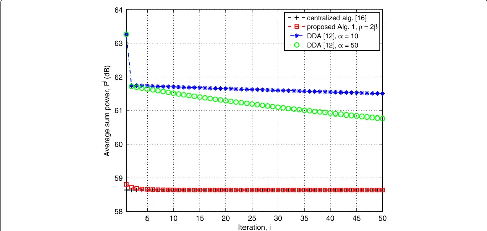
Figure 5 shows the average sum power versus iteration for multicell network 1a. The SINR targetγl is set to 15
dB for alll ∈ L. For a comparison, we consider central-ized algorithm [16, Section IV] and DDA [12]. DDA [12] plots are drawn for the subgradient step sizeα = 10, 50. For a fair comparison of Algorithm 1, DDA [12], and the centralized algorithm [16, Section IV], the plots are drawn for the fading realizations that are feasible for all consid-ered algorithms. Results show that the convergence speed of proposed Algorithm 1 compared with DDA [12] is fast and can achieves the centralized solution in less than ten iterations.
5 10 15 20 25 30 35 40 45 50
58 59 60 61 62 63 64
Iteration, i
Average sum power, P
i (dB)
centralized alg. [16] proposed Alg. 1, ρ = 2β DDA [12], α = 10 DDA [12], α = 50
0 5 10 15 40
45 50 55 60 65
SINR
Average sum power, P
i (dB)
centralized alg. [16] proposed Alg. 1, iter. = 20 proposed Alg. 1, iter. = 50
Figure 6Multicell network 2: Average sum power versus SINR.Multicell network 2: Average sum power versus SINR forρ=2β.
Figure 6 shows the average sum power versus SINR target for multicell network 1b. For a comparison, we con-sider centralized algorithm [16, Section IV]. To note a fair progress of the proposed algorithm for a wide SINR target values, each curve is averaged for the fading realizations that are feasible for all the SINR values. Plots are drawn for the average sum power at iteration number 10 and 50. Results show that the proposed Algorithm 1 can achieve the centralized solution over the wide rage of SINR target values.
We next evaluate the performance of Algorithm 3 for SINR balancing problem (P2). We, first, consider single fading realization and run the algorithm for both networks shown in Figure 1. As a benchmark, we consider central-ized optimal algorithm proposed in [16, Section V]. In the simulation, we set SNR = 5 dB, and for Algorithm 2, we set =0.1, andαnmax=2×100.1×SNRfor alln∈N. Plots are drawn forρ=0.5, 1, 2.
Figure 7 shows the progress of the global variableγ by iteration. Note that the global variableγ is the average of
5 10 15 20 25 30 35 40 45 50 −6
−4 −2 0 2 4 6
Iteration, i
γ
i (dB)
centralized alg. [16] proposed Alg. 3, ρ=0.5 proposed Alg. 3, ρ=1 proposed Alg. 3, ρ=2
(a)
10 20 30 40 50 60 70 80 90 100 −12
−10 −8 −6 −4 −2 0 2 4 6 8
Iteration, i
γ
i (dB)
centralized alg. [16] proposed Alg. 3, ρ=0.5 proposed Alg. 3, ρ=1 proposed Alg. 3, ρ=2
(b)
5 10 15 20 25 30 35 40 45 50 −6
−4 −2 0 2 4 6
Iteration, i
Feasible SINR,
γbest
(dB)
centralized alg. [16] proposed Alg. 3, ρ=0.5 proposed Alg. 3, ρ=1 proposed Alg. 3, ρ=2
(a)
10 20 30 40 50 60 70 80 90 100 −12
−10 −8 −6 −4 −2 0 2 4 6 8
Iteration, i
Feasible SINR,
γ
(dB)
centralized alg. [16] proposed Alg. 3, ρ=0.5 proposed Alg. 3, ρ=1 proposed Alg. 3, ρ=2
(b)
Figure 8Evolution of an average best SINR, that is feasible for all BSs.Feasible SINRγbesti versus iteration for SNR=5 dB:(a)Multicell network 1;(b)Multicell network 2.
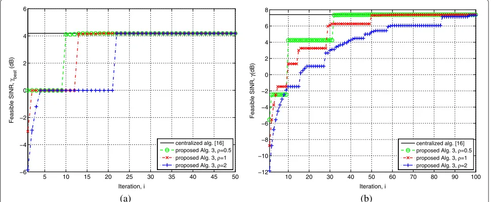
SINR values{αn}n∈Nthat is obtained independently by all NBSs (see (51)). Results show that for all considered val-ues ofρ, Algorithm 3 can obtain SINRγ that converges to the optimal centralized solution. Sinceγ is the average of the SINR values obtained independently in allN BSs, the intermediate values ofγ may not be feasible for all BSs before the algorithm converges. For example, the value of
γ for ρ = 0.5 is clearly infeasible at the iteration step i = {4, 5, 6, 7, 8}in Figure 7a. Therefore, to illustrate the convergence of feasibleγ, we define the following metric
γbesti = max t=1,...,i{γ
t
feas}, (56)
where γbesti is the best feasible SINR value at ith itera-tion, and γfeast is the feasible SINR attth iteration (53). Figure 8 shows the behavior ofγbesti by iteration. Results show that Algorithm 3 can obtain the feasible values of
γ that converges to the centralized solution. For example, withρ = 0.5, the algorithm converges to the centralized solution in just tenth iterations in Figure 8a.
Figure 9 shows the SINR γbesti for different SNR val-ueso. Each curve is averaged over 300 fading realizations. In the simulation, penalty parameterρis set to 0.5. Plots are drawn for the SINR obtained at iteration number 20, 30, and 50 of Algorithm 3. Results show that the proposed
−10 −8 −6 −4 −2 0 2 4 6 8 10 −10
−5 0 5
SNR (dB)
Average feasible SINR,
γbest
i
(dB)
centralized alg. [16] proposed Alg. 3, iter. = 20 proposed Alg. 3, iter. = 30 proposed Alg. 3, iter. = 50
(a)
−10 −8 −6 −4 −2 0 2 4 6 8 10 −6
−4 −2 0 2 4 6 8 10 12
SNR (dB)
Average feasible SINR,
γbest
i
(dB)
centralized alg. [16] proposed Alg. 3, iter. = 20 proposed Alg. 3, iter. = 30 proposed Alg. 3, iter. = 50
(b)
Algorithm 3 can achieve close to the centralized solution over the wide range of SNR values without any tuning ofρ.
6 Conclusion
We have provided distributed algorithms for the radio resource allocation problems in multicell downlink multi-input single-output systems. Specifically, we have con-sidered two optimization problems: P1 - minimization of the total transmission power subject to signal-to-interference-plus-noise ratio (SINR) constraints of each user, and P2 - SINR balancing subject to total transmit power constraint of BSs. We have proposed consensus-based distributed algorithms, and the fast solution method via alternating direction method of multipliers. First, we have derived a distributed algorithm for problem P1. Then, in conjunction with the bracketing method, the algorithm is extended for problem P2. Numerical results show that the proposed distributed algorithms converge very fast to the optimal centralized solution.
Endnotes
a Similar assumptions are made, e.g., in [36] in the
context of arbitrary wireless networks.
b The value ofR
intis chosen such that the power of the interference term is below the noise level, and this commonly used approximation is made to avoid unnecessary coordinations between distant BSs. The appropriate value ofRintcan be chosen to trade off between the required backhaul signaling and the
optimality of the solution. The effect of nonzeroznlterms can be accurately modeled by changing the statistical characteristics of noisenlat rec(l). However, those issues are extraneous to the main focus of the paper.
c In problem (4) and (5), the set{z
nl}l∈Lint,n∈Nint(l)is a
collection ofznlfor which thelth user is inside the interference region of BSn. Thus, the constrained for unconsidered out-of-cell interference term (i.e.,z2nl=0) forlth user that is outside the interference region of BSn is dropped in problem (4) and (5).
d A more general SINR balancing problem which can
set priority of users (keeping the SINR values of data stream to a fixed ratios) [6, Section IV-C] can be formulated. To simplify the presentation, we consider maximization of the minimum SINR. Note that the proposed decentralized method can be easily generalized to the more general problem considered in
[6, Section IV-C].
e Note thatL
int(n)⊆L(n). Hence, tran(l)=nfor all l∈Lint(n).
f To simplify the presentation, here we have used a
slight abuse of notation, i.e., we have considered that the sets in (12) are ordered.
gLet{u
k,nl}k∈{n,tran(l)},l∈Lint,n∈Nint(l)be the dual variables
associated with the equality constraints of problem (8),
then by following steps (10) to (12), one can easily express
un= {{un,nl}l∈Iint(n),{un,bl}l∈Lint(n),b∈Nint(l)},n∈N.
h Variablez
nl(component ofzn) couples two local variablesxn,nl(component ofxn) andxtran(l),nl
(component ofxtran(l)). Hence, in step (19) to updateznl coordination between BSnand BS tran(l)is required.
iFor convenience, we can combine the linear and
quadratic terms of problem (21) asuiTn (xn−zin)+
n}n∈Nare the dual variables associate with the consistency constraints of problem (16). By following steps (10) to (12), we can easily showun=
lIn ADMM algorithm, standard stopping criteria is to
check primal and dual residuals [21]. However, it is often the case that ADMM can produce acceptable results of practical use within a few tens of iteration [21]. As, finite number of iteration is more favorable for practical implementation, we adopt fixed number of iteration to stop the algorithm.
m For convenience we can combine the terms in
problem (40) as a)uiTn (xn−zin)+ ρ2xn−zin22=
n In ADMM algorithm, standard stopping criteria is to
check primal and dual residuals [21]. However, it is often the case that ADMM can produce acceptable results of practical use within a few tens of iteration [21]. As, finite number of iteration is favorable for practical
implementation, we adopt fixed number of iteration to stop the algorithm.
o For fixed radiusR
BSin Figure 1, different SNRs (i.e., different SNR(RBS)) are obtained by changingp
max 0
σ2 in (54).
pThe interval [0,αmax
n ] denotes the range of feasibleαn for problem (46).
Appendices
Appendix 1
In this appendix, we propose the bracketing method [30,31] to solve problem (44). Let us start by combining the second (linear) and third (quadratic) terms of (45) as
p(αn)= ˜p(αn)+
Without loss of generality, let us drop the constant term of (57) and simplify it as
p(αn)= ˜p(αn)+
ρ
2(αn−θ )
whereθ =γi−λin+ρ1N.
Note that the optimal value p˜(αn) is nondecreasing function ofαn ∈ [0,αmaxn ]p.To see that, letPi andPjbe the feasible set of problem (46) forαn = αni andαn = αn, respectively. Ifj αnj ≥ αin, then it is easy to see that
Pj ⊆ Pi. Hence, the optimal valuep˜(αnj) ≥ ˜p(αin)for all
αnj ≥αinandαin,α j
n ∈[0,αmaxn ]. Furthermore, there exists a partition of [0,αnmax] as [0,φ]∪[φ,αnmax] such that
˜
p(αn)=c, αn∈[0,φ] , (59)
wherecis the optimal solution of problem (46) forαn=0. Next, we propose to use bracketing method [30,31] to find the infimum of functionp(αn)on the intervalαn ∈ [0,αnmax]. First, in Lemma 1, we show that the function p(αn)is a unimodal function on the intervalαn∈[0,αmaxn ] for the condition: C)θ ≤φ.
Lemma 1.The function p(αn),
p(αn) = ˜p(αn)+ ρ
2(αn−θ )
2, (60)
is a unimodal function on the intervalαn ∈[0,αnmax]for the condition C.
Proof:
1. For the caseθ ≤0, the proof is trivial, sincep(αn)is a sum of two increasing functions on the interval αn∈[0,αmaxn ].
2. For the caseθ >0, let us partition[0,αnmax]as [0,θ]∪[θ,αnmax]. On the intervalαn∈[0,θ], the functionp˜(αn)takes a constant valuec. On the intervalαn∈[θ,αnmax], the functionp˜(αn)is a nondecreasing function. Hence, the functionp(αn) is a sum of affine and convex functions on the interval[0,θ], and a sum of nondecreasing and increasing functions on the interval[θ,αnmax]. Thus, the functionp(αn)is a unimodal function.
Lemma 1 implies that for the condition C (i.e., θ ≤ φ), the infimum of the function p(αn) can be obtained optimally by using bracketing method [30,31].
For the case condition C is not satisfied (i.e.,φ ≤ θ), let us partition [0,αmaxn ] as [0,φ]∪[φ,θ]∪[θ,αnmax]. On the intervalαn ∈[0,φ], the functionp(αn)is a decreas-ing function (since p˜(αn) takes a constant value c, and
(αn−θ )2is a decreasing function). On the intervalαn ∈ [θ,αmaxn ], the function p(αn) is an increasing function (sincep˜(αn) is nondecreasing function and(αn−θ )2 is increasing function). On the intervalαn ∈[φ,θ], analyt-ically expressing the curvature ofp(αn)is difficult, since the curvature of functionp˜(αn) depends on the numer-ical parameters. This implies that for the case φ ≤ θ,
the infimum of the function p(αn) lies on the interval [φ,θ], i.e.,
arg min
αn∈[0,αnmax]
p(αn)∈[φ,θ] . (61)
Thus in the caseφ ≤ θ (i.e., if condition C is not sat-isfied), the solution of problem (61) obtained by using bracketing method [30,31] lies at most(θ−φ)away from the optimal solution. However, in all of our numerical sim-ulations, we have always noted that the functionp(αn)is a unimodal function. In that case, problem (61) is solved optimally by bracketing method [30,31]. Moreover, the convergence of the proposed Algorithm 3 (see numerical example, Section 5) to the centralized solution shows that bracketing method can be used to solve problem (44).
Appendix 2
The ADMM method is guaranteed to converge for all values of its penalty parameter ρ [21]. However, the rate of convergence of ADMM algorithm is sensitive to the choice of the penalty parameter ρ. In practice, the ADMM penalty parameterρ is either tuned empirically for each specific application, or set equal to 1 by normal-izing the problem data set [21, Chapter 11]. Note that in Algorithm 1, to solve the local variable update (22), we can normalize the problem data (i.e., sum power
(l∈L(n)ml22))by normalizing factorβn > 0 and set
ρ = 1, which is equivalent to setρ = βnin Algorithm 1, if the problem data (i.e., sum power (l∈L(n)ml22)) is not normalized. To elaborate further, let us express equivalently the local variable update (22) as
minimize 1
βn ⎛
⎝
l∈L(n) ml22
⎞
⎠+ ρ
2xn−z i n+vin22
subject to
⎡ ⎢ ⎢ ⎢ ⎢ ⎢ ⎣
1+γ1
lh
H
llml
MHnhll ˜
xl
σl
⎤ ⎥ ⎥ ⎥ ⎥ ⎥
⎦SOC
0, l∈L(n)
xn,nl
MHnhjl
SOC 0, l∈Iint(n)
(62)
with variablesMn = [ml]l∈L(n) and xn, where βn > 0 is the normalizing factor,x˜l = {xn,bl}b∈Nint(l) is a subset
generalized inequalities with respect to the second-order cone [16,19].
For problem (62), the optimal choice of βn is
l∈L(n)ml22. However, before the convergence of Algorithm 1, we do not have optimal beamformers (i.e., {m
l}l∈L(n)). Thus, in our simulation, to estimateβn, we ignore the interference and noise terms and find beam-forming vectorm˜lthat achieves the required SINR thresh-oldγl, which can be expressed as
˜
ml =
100.1×γl/h
ll22, l∈L(n).
Hence, the normalizing factorβnfor problem (62) can be written as
βn=
l∈L(n) ˜
ml
=
l∈L(n)
(100.1×γl)/h
ll22.
Furthermore, we findβ = max
n∈N{βn}, and setρ = βfor
Algorithm 1.
Competing interests
The authors declare that they have no competing interests.
Acknowledgements
This research was supported by the Finnish Funding Agency for Technology and Innovation (Tekes), Nokia Solutions and Networks, Anite Telecoms, Renesas Mobile Europe, and Elektrobit.
Received: 14 April 2013 Accepted: 16 December 2013 Published: 4 January 2014
References
1. M Bengtsson, B Ottersten, Optimal Downlink Beamforming Using Semidefinite Optimization, inProceedings of the Annual Allerton Conference on Communications, Control, and Computing, (Urbana-Champaign IL, 1999), pp. 987–996
2. F Rashid-Farrokhi, KJR Liu, L Tassiulas, Transmit beamforming and power control for cellular wireless systems. IEEE J. Select. Areas Commun.16(8), 1437–1450 (1998)
3. E Visotsky, U Madhow, vol. 1, Optimum Beamforming Using Transmit Antenna Arrays, inProceedings of the IEEE Vehicular Technology Conference, (Houston, TX, 1999), pp. 851–856
4. Q Shi, M Razaviyayn, M Hong, ZQ Luo, SINR constrained beamforming for a MIMO multi-user downlink system, inProceedings of the Annual Asilomar Conference on Signals, Systems and Computers, (Pacific Grove, CA, 2012), pp. 1991–1995
5. KK Wong, G Zheng, TS Ng, vol. 1, Convergence analysis of downlink MIMO antenna systems using second-order cone programming, inProceedings of the IEEE Vehicular Technology Conference, (Dallas, 2005), pp. 492–496 6. M Codreanu, A Tölli, M Juntti, M Latva-aho, Joint design of Tx-Rx
beamformers in MIMO Downlink channel. IEEE Trans. Signal Process.
55(9), 4639–4655 (2007)
7. M Schubert, H Boche, Solution of the Multiuser downlink beamforming problem with individual SINR constraints. IEEE Trans. Vehic. Technol.53, 18–28 (2004)
8. H Boche, M Schubert, Optimal multi-user interference balancing using transmit beamforming. Wireless Pers. Commun., Kluwer Acad. Publishers.
26(4), 305–324 (2003)
9. M Schubert, H Boche, Comparison of∞-norm and1-norm optimization
criteria for SIR-balanced multi-user beamforming. Elsevier Signal Process.
84(2), 367–378 (2004)
10. A Tolli, M Codreanu, M Juntti, Minimum SINR maximization for multiuser MIMO downlink with per BS power constraints, inProceedings of the IEEE Global Telecommunication Conference, (Kowloon, 2007), pp. 1144–1149 11. HDW Yu, Coordinated beamforming for the multicell multi-antenna
wireless system. IEEE Trans. Wireless Commun.9(5), 1748–1759 (2010) 12. A Tölli, H Pennanen, P Komulainen, Decentralized minimum power
multi-cell beamforming with limited backhaul signaling. IEEE Trans. Wireless Commun.10(2), 570–580 (2011)
13. H Pennanen, A Tolli, A Latva-ahom, Decentralized coordinated downlink beamforming via primal decomposition. IEEE Signal Process. Lett.18(11), 647–650 (2011)
14. D Nguyen, T Le-Ngoc, Multiuser downlink beamforming in multicell wireless systems: a game theoretical approach. IEEE Trans. Signal Process.
59(7), 3326–3338 (2011)
15. C Shen, T Chang, K Wang, Z Qiu, C Chi, Distributed robust multicell coordinated beamforming with imperfect CSI: an ADMM approach. IEEE Trans. Signal Process.60(6), 2988–3003 (2012)
16. A Wiesel, YC Eldar, S Shamai, Linear precoding via conic optimization for fixed MIMO receivers. IEEE Trans. Signal Proc.54, 161–176 (2006) 17. S Boyd, L Xiao, A Mutapcic, J Mattingley, Notes on decomposition
methods: course reader for convex optimization II, Stanford 2007. [[Online]. Available: http://www.stanford.edu/class/ee364b/notes/ decomposition_notes.pdf]. Accessed 01 March 2012
18. S Boyd, Subgradient methods 2007. [[Online]. Available: http://www. stanford.edu/class/ee364b/lectures/subgrad_method_slides.pdf]. Accessed 01 March 2012
19. S Boyd, L Vandenberghe,Convex optimization(Cambridge University Press, Cambridge, 2004)
20. Y Huang, G Zheng, M Bengtsson, KK Wong, L Yang, B Ottersten, Distributed multicell beamforming with limited intercell coordination. IEEE Trans. Signal Process.59(2), 728–738 (2011)
21. S Boyd, N Parikh, E Chu, B Peleato, J Eckstein, Distributed optimization and statistical learning via the alternating direction method of multipliers. Foundations Trends Mach. Learn.3, 1–122 (2010)
22. J Yang, Y Zhang, Alternating direction algorithms for1-problems in
compressive sensing. SIAM J. Sci. Comput.33, 250–278 (2011) 23. M Figueiredo, J Bioucas-Dias, Restoration of poissonian images using
alternating direction optimization. IEEE Trans. Image Process.19(12), 3133–3145 (2010)
24. I Schizas, A Ribeiro, G Giannakis, Consensus in ad hoc WSNs with noisy links-part I: distributed estimation of deterministic signals. IEEE Trans. Signal Process.56, 350–364 (2008)
25. M Leinonen, M Codreanu, M Juntti, Distributed consensus based joint resource and routing optimization in wireless sensor networks, in
Proceedings of the Annual Asilomar Conference on Signals, Systems and Computers, (Pacific Grove, CA, 2012)
26. B He, X Yuan, On theO(1/n)convergence rate of the Douglas-Rachford alternating direction method. SIAM J. Numerical Anal.50(2), 700–709 (2012)
27. J Mota, J Xavier, P Aguiar, M Puschel, Distributed ADMM for model predictive control and congestion control, inProceedings of the IEEE International Conference on Decision and Control, (Maui, HI, 2012), pp. 5110–5115
28. W Deng, W Yin, On the global and linear convergence of the generalized alternating direction method of multipliers, inRice CAAM tech report TR12-14(2012)
29. M Hong, ZQ Luo, On the linear convergence of the alternating direction method of multipliers, inarXiv preprint arXiv:1208.3922, (2012) 30. JH Mathews, KK Fink,Numerical Methods Using Matlab, 4th edn
(Prentice-Hall Inc., Upper Saddle River, 2004)
31. W Cheney, D Kincaid,Numerical Mathematics and Computing, 4th edn (International Thomson Publishing, Stamford, 1998)
32. S Joshi, M Codreanu, M Latva-Aho, Distributed resource allocation for MISO downlink systems via the alternating direction method of multipliers, inProceedings of the Annual Asilomar Conference on Signals, Systems and Computers, (Pacific Grove, CA, 2012), pp. 488–493 33. DP Bertsekas,Constrained Optimization and Lagrange Multiplier Methods
34. D Bertsekas, J Tsitsiklis,Parallel and Distributed Computation: Numerical Methods(Athena Scientific, Belmont, 1997)
35. A Kumar, D Manjunath, J Kuri,Wireless Networking(Elsevier Inc., Burlington, 2008)
36. P Gupta, PR Kumar, The capacity of wireless networks. IEEE Trans. Inform. Theory46(2), 388–404 (2000)
doi:10.1186/1687-1499-2014-1
Cite this article as:Joshiet al.:Distributed resource allocation for MISO downlink systems via the alternating direction method of multipliers. EURASIP Journal on Wireless Communications and Networking20142014:1.
Submit your manuscript to a
journal and benefi t from:
7Convenient online submission
7Rigorous peer review
7Immediate publication on acceptance
7Open access: articles freely available online
7High visibility within the fi eld
7Retaining the copyright to your article