Volume 2009, Article ID 804021,16pages doi:10.1155/2009/804021
Research Article
Mobile Station Spatio-Temporal Multipath Clustering
of an Estimated Wideband MIMO Double-Directional Channel
of a Small Urban 4.5 GHz Macrocell
Lawrence Materum,
1Jun-ichi Takada,
1Ichirou Ida,
2and Yasuyuki Oishi
21Takada Laboratory, Department of International Development Engineering, Graduate School of Science and Engineering,
Tokyo Institute of Technology, 2-12-1-S6-4, O-okayama, Meguro-ku, Tokyo 152-8550, Japan
2Fujitsu Limited, 5-5 Hikari-no-oka, Yokosuka, Kanagawa 239-0847, Japan
Correspondence should be addressed to Lawrence Materum,[email protected]
Received 2 August 2008; Revised 11 December 2008; Accepted 5 February 2009
Recommended by Michael A. Jensen
Multipath clusters in a wireless channel could act as additional channels for spatial multiplexing MIMO systems. However, identifying them in order to come up with better cluster channel models has been a hurdle due to how they are defined. This paper considers the identification of these clusters at the mobile station through a middle ground approach—combining a globally optimized automatic clustering approach and manual clustering of the physical scatterers. By including the scattering verification in the cluster identification, better insight into their behavior in wireless channels would be known, especially the physical realism and eventually a more satisfactorily accurate cluster channel model could be proposed. The results show that overlapping clusters make up the majority of the observed channel, which stems from automatic clustering, whereas only a few clusters have clear delineation of their dispersion. In addition, it is difficult to judge the physical realism of overlapping clusters. This further points to a need for the physical interpretation and verification of clustering results, which is an initial step taken in this paper. From the identification results, scattering mechanisms of the clusters are presented and also their selected first and second order statistics.
Copyright © 2009 Lawrence Materum et al. This is an open access article distributed under the Creative Commons Attribution License, which permits unrestricted use, distribution, and reproduction in any medium, provided the original work is properly cited.
1. Introduction
The clustering of multipaths has started to be considered as an aspect of multiple-input multiple-output (MIMO) propagation channel models [1–3]. Given that they exist and depending on the target MIMO application, accurate knowledge of them in the channel is one of the ways to take advantage of the benefits of MIMO systems, especially that of spatial multiplexing systems, wherein these clusters could act as additional channels. Characterizing multipath clusters should therefore be satisfactorily accurate and this hinges on the reality of these clusters. This starts by identifying them appropriately. Many previous studies (e.g., [1,4–7]) identified multipath clusters manually/visually after some preprocessing. Manual clustering approaches are the majority of the methods used in identifying multipath clusters. Distinct from these manual clustering approaches are automatic clustering approaches [8–11], which on the
other hand are the minority. These automatic clustering approaches were made in response to the cumbersomeness of identifying clusters manually from large estimated channel data derived from channel sounding. Table 1 shows a comparison of these two approaches. Each approach has its own strengths and weaknesses. One big deficiency of current automatic clustering approaches is their lack of physical realism, that is, the multipath clustering results may not correspond to physical objects in the environment, thus they may just be numerical and inaccurate. In contrast, manual approaches could check the physical validity of the clustering results.
Table 1: Comparison of two multipath cluster identification approaches.
Automatic clustering Manual clustering
– real-world clusters are complicated – unwieldy and subjective
– mathematically trackable – physically trackable
– number-based – object-based
– “better” number processor – “better” object processor
Table2: Medav-RUSK-Fujitsu wideband MIMO channel sounder.
Carrier frequency 4.5 GHz
Bandwidth 120 MHz
BS antenna
Uniform rectangular array
2×4×2 elements (row×col.×pol.)
V & H polarized patch antennas
MS antenna
Stacked uniform circular array
2×24×2 elements (row×col.×pol.)
V & H polarized patch antennas
Transmit signal Wideband multitone
Maximum delay setting 3.2μs
Number of MIMO channels 1536
Table3: Small urban macrocell scenario.
BS height ∼85 m
MS height ∼1.80 m
BS-MS distance ∼230–400 m
Structure type residential & industrial
of multipath clusters. However, the specific focus of this paper is to identify clusters more effectively. The outcomes consisted of overlapping clusters, which was attributed to automatic clustering, and clusters with clear delineation, attributed to the manual clustering approach. The result demonstrates the need for the physical interpretation and validation of automatic clustering results, which is an initial step done in this paper. This paper is structured then as follows. In Section 2, the source of the estimated MIMO channel data is described. This is followed by an overview of the approach inSection 3. The details of the approach are discussed in Sections3.1and3.2, which refer to automatic and manual multipath clustering, respectively. Sections 2–
3.2comprise the highlighted part of the framework behind this paper as portrayed inFigure 1. After these sections, the results and subsequent discussions are laid out inSection 4. Finally, conclusions are summarized and drawn.
2. Estimated MIMO Channel
After a macrocell site survey and planning for a mea-surement campaign in Kawasaki City, Kanagawa, Japan, channel sounding was performed using the Medav-RUSK-Fujitsu MIMO channel sounder [12]. Pertinent details of this wideband channel sounder and the measurement site are in described in Tables2and3, respectively. The array antennas
Macrocell site survey and
planning for measurement
campaign
Channel sounding and parameter
estimation
Middle ground multipath clustering
Manual multipath clustering
Automatic multipath clustering
Number of multipath clusters: average rank aggregation
Global optimization: simulated annealing Local optimization: K-means clustering
MIMO channel analysis
and modeling (not included in this paper)
Figure1: Overall framework. The prominent group presented in this paper shows the progression of the middle ground multipath clustering approach from the automatic clustering optimization to manual multipath clustering.
that were used were carefully calibrated in an anechoic chamber, which is important for path parameter estimation [13,14]. A map of the small urban macrocell showing the base station (BS) and mobile station (MS) positions is shown inFigure 2. Photographs of selected positions are shown in
Figure 3. With this measurement setup, time snapshots of the channel were taken after midnight under a clear spring weather while the MS was moved at a slowly walking pace along the street. In between MS positions, the MS movement covers a 20 m length route, starting and ending with static measurements.
A maximum likelihood multidimensional parameter estimation algorithm was used to extract the delay (τ), azimuth (φ), and co-elevation (θ) angle of departure (AoD),
φ and θ angle of arrival (AoA), and the four complex polarimetric weights (γVV,γVH,γHV,γHH) including the
dif-fuse components [15, 16], where V and H denote the vertical polarization and horizontal polarization, respec-tively. Briefly, the co-elevation angle is referred to here as the elevation angle. The estimation algorithm is based on the double-directional channel concept, which makes the results independent of the antennas used [17]. The measurement site and the estimated channel are precursors to the multipath clustering progression described inFigure 1.
3. Bicombinational Multipath Clustering
BS
BS direction
St
reet di
recti
on
Facing BS direction MS
MS MS
MS MS
MS MS
MS MS
MS MS
MS MS
MS MS
MS MS MS MS MS
N
100 m
© Copyright ZENRIN Co., LTD.
Figure2: BS and MS positions in the measurement site. The BS antenna was placed on top of a building which was the highest one
in that location (Figure 3(c)), whereas the MS positions were along
the street. The average height of the buildings around the BS was less than half its height.
seen to operate like “group of patterns are seen, therefore they are clusters,” whereas for automatic clustering “group of patterns are numerically optimized, so they are clusters.” Thus, one approach depends on what is seen, but the other on numbers. Visual reliance per se or numerical reliance per se tend to focus only on their respective results. The approach of this paper tries to combine the strengths of each view.
Given the backdrop notion that modeling clusters starts by their correct identification, three factors were considered in the middle ground clustering approach. These factors are listed inTable 4.
In this paper, the multidimensional Euclidean distance was used primarily as the similarity/dissimilarity measure (seeSection 3.1), whereas for the significance measure, clus-ters were considered primarily by their power (specifically, power proportion; see Section 4.1), and for the validation measure, they were verified: (i) numerically by the average rank aggregation (Section 3.1.3) of their clustering validity indices, and (ii) manually by their corresponding or asso-ciated scatterers and propagation mechanisms. It is noted that this is an important step in validating clusters produced by automatic clustering as it connects with the physical environment. It has been observed that this validation is lacking in many existing publications on multipath clusters.
A middle ground approach developed inductively from employing each view [18, 19], and then both views are presented here. In the automatic clustering side, a locally optimal clustering algorithm was used together with a stochastically global optimization strategy. The results of the
(a) A view from the BS
(b) A view from an MS position near the southeast side ofFigure 2
BS
(c) A view of the BS from an MS position
Figure3: Views of the measurement site.
Table4: Factors considered in the middle ground clustering approach.
Factor Possible quantification Gives an answer to
Similarity/dissimilarity measure Multidimensional distance, probability
density function,. . .
How near/far are multipaths from each other?
Significance measure Shape, size, power, mutual information,
target application performance,. . . Which multipaths are considered?
Validation measure Clustering validity index, physics,
scatterers,. . . How are the identified clusters validated?
Before presenting the details of the multipath clustering approach in Sections 3.1, 3.2, other related aspects of processing the estimated channel are described as follows.
Preprocessing. The clustering was done jointly in all the
spatial and temporal dimensions of the channel parameters. Thelth path channel data for clustering is denoted here as
Xl=
τl φAoDl θAoDl φAoAl θlAoA
, (1)
which represent the delay and direction dimensions. Before automatic clustering was performed, the angular data inX
were first transformed to their direction cosines in order to transform them into a linear scale. Thus dim{X} = 7 as a result of mapping the two-unit spherical dimensions (azimuth and elevation) to three-unit Cartesian dimen-sions (S2 → R3). Included with this preprocessing is
the normalization or scaling of each dimension in X to have zero mean and unit variance. Further, the strongest paths that represent the line of sight (LoS) were removed using the single path estimate. This was based on the goal of only modeling clusters that are due to multipath mechanisms. It also follows the identification framework proposed in [20], where the LoS component is subtracted. In addition, six snapshots of every MS position shown in
Figure 2were combined for automatic clustering. This six-snapshot frame corresponds to a physical distance of about 2.5 m, which is the resolution of the channel sounder. This snapshot framing was done for all the snapshots in an MS position. Dynamic parameters are not considered in this paper, so only a static six-snapshot frame of every MS position were used. Furthermore, because of the limitations of the channel sounder for dynamic outdoor measurements, the Doppler dimension was not included. Specifically, the storage system of the channel sounder could not write as fast as the system measures the next Doppler block due to the time length in processing the buffered data before storage. Furthermore, it was not feasible to reduce the number of antenna elements at the BS and MS, and also the number of frequency bins in order to match the rate of the storage system.
Pruning. After determining the number of multipath
clus-ters, cluster pruning was performed as suggested in [9]. The pruning was done simultaneously in six dimensions. These dimensions are the cluster power, the root-mean-square (rms) delay spread, and the rms spreads of theφandθAoDs
and AoAs. In the multipath cluster pruning implementation, all paths run into a loop. In that loop, a path is pruned if all the remaining cluster power and clusters spreads without it are≥99% of the unpruned cluster power and rms spreads.
Propagation Mechanism Classes. As was done in [1,4,21], different propagation mechanism classes were considered, which are also adopted here. These propagation mechanism classes basically depend on the layout of the measurement. Thus they belong to the property of the scatterers in the environment. The considered propagation mechanism classes are (i) BS direction, (ii) facing BS direction, and (iii) street direction classes. Each one is divided further into two: (a)roof directionand (b)ground directionclasses. Knowing these propagation mechanisms classes could show how multipath clusters are related to the measurement site. These classes are based on the direction where a cluster comes from as seen at the MS. Figure 2 roughly shows these directions. Since the viewpoint was at the MS, the street direction was used as a reference in determining the BS direction and facing BS direction. So the BS direction refers to those multipaths whose azimuth AoAs come from the left side of the street, while those that are from the right side are the facing BS directions. The limiting 86-degree field-of-view of the MS patch antennas was used to determine the extent of the street direction region. From the estimated MIMO channel data, the azimuth AoA reference was placed at 0◦. This reference was parallel to the street direction for all the MS positions. For the elevation propagation mechanism classes, the roof direction classes are those multipaths whose co-elevation AoAs are above the MS (θ < 90◦), and otherwise for the ground directions.
3.1. Automatic Multipath Clustering. The local and global
optimizations done in solving the multipath clustering problem, and the evaluation of the number of multipath clusters are described in what follows.
[9, 10]. The K-means clustering algorithm gives a locally optimal solution to a nondeterministic polynomial-time-hard (NP-polynomial-time-hard) problem [23–26]:
minimize
K
k=1 L
l=1
Vkld
Xl,µk
subject to
K
k=1
Vkl=1, Vkl∈ {0, 1},
(2)
where K is the number of clusters, Vkl is the assignment
indicator of Xl to thekth cluster (Vkl ∈ VK×L), µk is the
kth cluster centroid, andd(Xl,µk) is the distance measure
betweenXlandµk. As was mentioned, the multidimensional
Euclidean distance was used ford. The power was not used in weighing the distance measure in the K-means clustering implementation as was done in [9], because clustering result trials done by the authors converged to almost the same results. Moreover, it also lessens the computation time because of the use of simulated annealing (Section 3.1.2). Using the distance measure on the dimensions ofX, a cluster is then seen as a group of multipaths having similar delay and direction which are spread around a certain centroid.
K-means clustering with the multidimensional Euclidean distance was used instead of kernel-based K-means and/or spectral clustering methods [27]. Though admittedly these methods could group nonconvex-shaped clusters, as opposed to multidimensional Euclidean K-means, the deter-mination of the tuning parameters that these approaches use is not straightforward. In the end, nonconvex multipath clusters could be more complicated to model, given that they have been verified to physically exist and are significant. In this paper, K-means clustering, which is a partitional way of clustering, was used because it is dynamic in moving
Xl’s from one cluster to another [28]. This is in contrast
to hierarchical clustering methods (e.g., single-linkage [11]), which are static in the sense that Xl’s assigned to a cluster
cannot be moved to other clusters in later iterations to minimize the objective function [28]. Using K-means to solve (2) is an expectation-maximization (EM) variation in the hard sense [29].
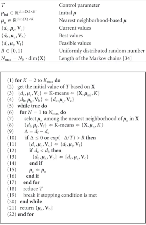
3.1.2. Globally Optimal Clustering. Equation (2) is an opti-mization problem and its objective function could have many local minima. It is a combinatorial minimization problem where K-means is only able to guarantee locally optimal solutions, that is, in general its result is one among the local minima and may not be the global minima. Using simulated annealing, this local minima feature of K-means could be cir-cumvented at the price of expensive computation. Simulated annealing is a globally stochastic optimization strategy that is conceptually a Monte Carlo method modeled according to physical annealing from statistical mechanics [30], which is a form of the Metropolis-Hastings algorithm [31,32]. It has been used in various combinatorial optimization problems and has been also successful in circuit and antenna array design problems [30, 33]. A pseudocode using simulated annealing with clustering is shown inTable 5.
The statistical polynomial-time cooling schedule [34] was used for the initial value and reduction of the control parameter T, and also for the stopping condition. Using this cooling schedule, the initial value ofT was iteratively calculated through several Markov chains using (3) until the initial acceptance ratioχ0is achieved. Hereχ0was set to 0.9:
Tini=
Δd+ ln
m2
m2χ0−m1
1−χ0
−1
. (3)
In (3), m1, initially zero in the first Markov chain, is the
number of Markov transitions fromito j, wheredi dj;
m2, also initially zero, is the number of Markov transitions
fromitoj, wheredi< dj; andΔd+is the averageΔdform2 transitions (i.e.,Δd >0,Δd =dj−di). For the reduction of
Tat theith iteration, it was obtained as
Ti=Ti−1 1 + Ti−1
ln(1 +δ) 3σdTi−1
−1
, (4)
whereδis the decrement parameter, which was set to 0.1, and
σdTi−1 is the standard deviation ofdin the Markov chain at
Ti−1. Finally, convergence is reached when the stop criterion
dTTini∂
ds(T)
∂T
< (5)
is satisfied, whereds(T)is the smoothedd(T)over the
length of the Markov chains, whereasis the stop parameter, which was set to 1×10⁻³. The statistical polynomial-time cooling schedule is a thorough approach and theoretically based way of running simulated annealing as compared to empirical cooling schedules. For the theoretical basis of the control parameter cooling schedule, readers are referred to [34].
InTable 5,µini is randomly chosen fromX; however, it is further refined by the long Markov chains and the nearest neighborhood-based centroid selection. At most, 30 nearest neighborhood paths ofµc inXwere the candidates for the random selection ofµn. The closeness was measured using the multidimensional Euclidean distance. In the same table, the constant N0 was set to 3, which was a compromise
between efficiency of the available computing resource and effectiveness of the simulated annealing implementation. It is noted that a deterministic cluster centroid initialization could also be used as was done in [35]. However, by virtue of the large search space of multipath centroids in running the K-means clustering algorithm inside simulated annealing, closer solutions to (2) are achieved because simulated annealing could jump away from being trapped in a local minima.
Table5: Clustering with simulated annealing pseudocode.
T Control parameter
µini∈Rdim{X}×K Initialµ
µn∈Rdim{X}×K Nearest neighborhood-basedµ
{dc,µc,Vc} Current values
{db,µb,Vb} Best values
{df,µf,Vf} Feasible values
R∈[0, 1) Uniformly distributed random number
Nmax=N0·dim{X} Length of the Markov chains [34]
(1)forK=2 toKmaxdo
(2) get the initial value ofTbased onX
(3) {dc,µc,Vc} ⇐K-means⇐ {X,µini,K}
(4) {db,µb,Vb} ⇐ {dc,µc,Vc}
(5) whiletruedo
(6) forN=1toNmaxdo
(7) selectµnamong the nearest neighborhood ofµcinX
(8) {df,µf,Vf} ⇐K-means⇐ {X,µn,K}
(18) reduceT
(19) break if stopping condition is met
(20) end while
(21) return{µb,Vb}
(22)end for
Algorithm1
the solid, and not to miss the lowest-energy state, otherwise the solid will become metastable. When the cooling is done this way, the solid could reach thermal equilibrium at each temperature. A large number of gradations is thus presented by the slow-cooling temperature schedule. This annealing process was simulated by [31] where the energy difference at each state of the solid is accepted when they reach thermal equilibrium, which could be described by the Boltzmann distribution. The temperature of the annealing process corresponds then to the control parameter T. So
Table 5 could then be concisely described by allowing K-means clustering to be run through long Markov chains, with sufficiently high initial T, which is then carefully decreased, the accepted solution to (2) approaches the global minima in the stochastic sense. In contrast to other clustering algorithms [8–11, 36], their results may only be locally optimal.
3.1.3. Number of Clusters (K). Determining the best K
is difficult because it requires a priori knowledge of the formation of multipath clusters in the environment, which
is not practically available. Nonetheless, it could be found by evaluating the clustering results using criteria set forth by clustering validity indices. These criteria are mainly based on cohesion (compactness) and separation measures of the clusters. So a clustering validity index tells the quality of clustering results that could give the best grouping. The indices that were used are described in what follows. These indices are optimizing in nature, that is, the maximum or minimum values of their arguments indicate the appropriate clustering.
(a)Silhouette Index. The Silhouette indexslkcould measure
how similar a multipath l is to all multipaths in its own clusterCkcompared to all multipaths of the cluster nearest
to it [37]. It is expressed as
Aslk=+1 means well-separated clusters whereas−1 signifies
the opposite. Following [8], the bestKcould be found as
KSI=arg max
(b) Davies-Bouldin Index. This index is a function of the
ratio of the intracluster separation sum (Si) to the intercluster
separation [38]. The bestKis found as
(c) Cali´nski-Harabasz Index. This index is a ratio of the
trace of the between-cluster scatter matrix to the trace of the within-cluster scatter matrix [39]. The bestKusing this index is
whereBandWare, respectively, given as
whereµis the global centroid of the estimated channel in an MS position.
The Davies-Bouldin index and Cali ´nski-Harabasz index were also used in [9]. Clustering algorithms that have basically the same objective function as that in (2) could result in being over-clustered or under-clustered as K is varied [40]. When the clustering results in either case, clus-tering validity indices that use intracluster and intercluster separation measures have a tendency to decrease or increase monotonically. This effect makes it difficult to determine the number of clusters. Moreover, the K’s determined by (9), (10), and (12) are based on the clustering results of only a single value of K considered in its argument. Instead of considering only a singleK, the Kim-Parks index [40], and the dynamic index [41] considered here give a validity that considers all the K’s used. Considering all theK’s used in a clustering validity index could avoid the monotone effect [40,41]. A disadvantage of using these two clustering validity indices is the increase in computation time.
(d) Kim-Parks Index. This index is a function of the sum
of (i) the total intracluster separation, as a measure of under-partition, and (ii) an over-partition function of the minimum distance between cluster centroids. Using it, the bestKis taken as
KKP=arg min K
1
K
k
Sk
+ K
arg mink=/k
dµk,µk
,
(14)
where each summand of the argument is normalized as
xarg=(x−xmin)/(xmax−xmin).
(e)Dynamic Index. This index tries to include the geometri-cal aspect ofXwhile taking into account the affinity of each cluster [41]. It determines the bestKas
KDI=arg min K
arg maxdµk,µk
arg mink=/k
dµk,µk
+ζ
K
l
kvar
Xl∈Ck
lvar
Xl
,
(15)
where
ζ= arg max
dXl,Xl
arg minl /=l
dXl,Xl·
lvar
Xl
l
2
k=1var
Xl∈Ck
,
(16)
whereas var(·) denotes the variance.
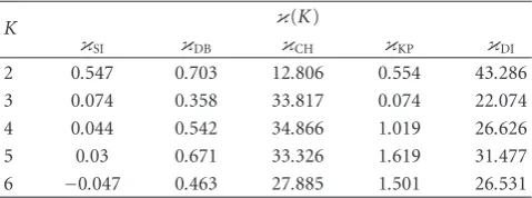
Average Rank Aggregation. For differentK’s, each argument inKSI,KDB,KCH,KKP, andKDI—denoted here byκ(K)—has
a different scale from one another, an example of which is shown inTable 6. Since theseκ(K)’s differ in evaluating the qualities of the clustering results, it is also not straightfor-ward to normalize them to one scale. To address these issues and to not only depend on one clustering validity index
Table6: Exampleκ(K) forK=2 toK=6.
K κ(K)
κSI κDB κCH κKP κDI
2 0.547 0.703 12.806 0.554 43.286
3 0.074 0.358 33.817 0.074 22.074
4 0.044 0.542 34.866 1.019 26.626
5 0.03 0.671 33.326 1.619 31.477
6 −0.047 0.463 27.885 1.501 26.531
Table7: Average rank aggregation applied to the data inTable 6.
K sr(κ)
srSI srDB srCH srKP srDI sr(∀sr)
2 5 1 1 4 1 2
3 4 5 4 5 5 5
4 3 3 5 3 3 4
5 2 2 3 1 2 1
6 1 4 2 2 4 3
result, the weighted voting aggregation of [42] was adopted but with a proposed modification: instead of scoringκ(K)’s by weighted votes, they are scored by their statistical rank— sr(κ). This removes the bias in the determination of the best
Kas it does not depend on the weights. The rank aggregation strategy is shown in Table 7 using the κ(K) example in
Table 6. The result suggests that the best K is 3 based on the highest sr(·) of the sr(κ) average of all clustering validity indices. The next highest sr(·)’s could be checked as well if the clustering result of the highest one does not meet the criteria. As a comparison, when weights are used and are determined optimally or heuristically, the use of the average rank aggregation strategy offers a significant reduction in the overall computation time.
3.2. Manual Multipath Clustering. Real-world clusters could have irregular shapes like nonspherical or nonellipsoidal multipaths groupings, which could be readily recognized by the human eye, but not automatically by mathematical algo-rithms [8]. Several aspects that contribute to this irregular shaping are the dimensionality of X and manifold cluster characteristics due to the physical environment. Accommo-dating functionalities, for example, contracting projections and separators [43], which address these shapes adaptively in the mathematical clustering algorithm would result in an inefficient algorithm. Thus, the authors consider that the human aspect should not be ignored in the cluster validation analysis, especially in the verification of the physical realism of the clustering of multipath estimates as was also similarly done in [1,4,6], and not just fully depend on mathematical clustering results. This validation then incorporates the so-calleddomain knowledge(from data-mining terminology) in validating clusters.
120
ElevationAoD (
◦)
ElevationAoD (
◦)
ElevationAoD (
◦)
(j)
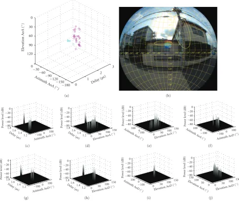
Figure4: Outcome of the clustering approach at one position of an MS measurement location.
the MS, corresponding scatterers of each cluster were visually identified. This was done by viewing the automatic clustering results in several dimensions in conjunction with fisheye photographs of the MS position where automatic clustering was performed. A fisheye image is basically a projection of a hemispherical image to a plane. The following criteria were used in verifying the results of automatic clustering:
(i) within-processing limitations, (ii) non-overlapping in delay, (iii) scatterer existence.
The channel sounder resolution is included in (i). For the case of using the multidimensional Euclidean K-means algorithm, its processing limitation results in verifying only observable convex-shaped clusters. The non-overlapping criterion was used in order to delineate clusters from paths that may not be part of it, thus keeping the verity of cluster dispersion. Delay overlap of the clusters was allowed only
in one dimension. As was done in [10], singleton clusters were not included as clusters since the results show that they have relatively weak power. However, it is also recognized that a singleton cluster could be considered as a cluster of rays if they have significant power [44]. When clusters have been verified, statistics are gathered such as their most likely scatterer type, the number of clusters, and the propagation mechanism class. This manual clustering is seen as an important step in validating clusters produced by automatic clustering as it connects with the physical environment, which is lacking in many existing publications on multipath clustering.
4. Results and Discussion
Applying the clustering approach presented in Section 3
to the estimated channel described in Section 2, Figure 4
shows one of the results. The automatic clustering result in
120
Figure5: Another example showing four multipath clusters.
inFigure 4(b). The cluster-scattering objects were attributed to the single-storey and two-storey concrete buildings. To further verify these two clusters, their power profiles were examined, which are shown in Figures4(c)–4(j). Comparing the plots in this figure, the two clusters are clearly seen in the azimuth-delay profiles than in the azimuth-elevation profiles due to the intersection of cluster elevation AoAs. These two clusters were not only observable at the MS and BS side through their azimuth-delay profiles but could also be confirmed through their AoA-AoD profiles (except slightly for the AoD profiles due to the closeness of the cluster elevation directions). Similarly,Figure 5shows a result with four multipath clusters. Two of the cluster-scattering objects were attributed to the asphalt road, whereas the other two were attributed to the concrete wall and concrete sidewalk. These results confirmed that the clustering approach was able to capture clusters that fall within its capability andlinebreak criteria.
Using the manual clustering criteria set forth in
Section 3.2 also resulted in clusters that were classified as
mathematical clusters, which are hereafter called α-clusters. Many of the clusters that fall into this category are those that overlap with other clusters in their scenarios, whereas others are singleton clusters. Among the criteria, the overlapping— in delay and/or direction—of these clusters was the main reason why they were classified asα-clusters.Figure 6shows an example of these clusters, where the overlapping of three clusters could be seen. Possible grounds for theseα-clusters are (i)other components(far clusters, clusters at the locality of the BS, nonclusters, dynamic paths, etc.), or (ii) errors
150
ElevationAoD (
◦)
ElevationAoD (
◦)
ElevationAoD (
◦)
(j)
Figure6: A mathematical clustering result—overlapping clusters.
Table8: Percentage of cluster propagation mechanism classes.
Classes Ground [%]a Roof [%]a Overall [%]a
Street direction 10.6316.93 12.213.39 22.8330.32
BS direction 5.127.09 6.35.12 11.4212.21
Facing BS direction 4.727.48 6.694.33 11.4111.81
aα-clusters/β-clusters.
This could also be examined in the AoA-AoD profiles in both the azimuth and elevation dimensions in Figures4(f),4(j),
5(f),5(j),6(f), and6(j). The narrowness of the AoD range spanned by the clusters in these power profiles indicates the absence of clustering at the BS side.
4.1. Power Proportion. Collecting the clustering results of the approach applied to the estimated MIMO channel data, the significance measure (seeSection 3) of the clusters are examined here in terms of their power proportion. The use
of power proportion as a measure of cluster significance has been also used in [6]. For a certain MS measurement location, this power proportion is defined here as the ratio of the cluster path power to the total path power. For a cluster
Ck, it is expressed as
Table9: Material-type percentage of theβ-cluster scatterers.
Material type Street direction BS direction Facing BS direction Overall [%]
Ground [%] Roof [%] Ground [%] Roof [%] Ground [%] Roof [%]
Metal 5.9 12.3 7.8 3.4 2 3.9 35.3
Concrete 8.8 6.9 3.9 2.9 6.9 1 30.4
Asphalt 15.2 − 0.5 − 1 − 16.7
Brick 0.5 5.8 − − 1 2 9.3
Mixed (metal, concrete, foliage, window) − 5.4 − − − 2.9 8.3
0 0.1 0.2 0.3 0.4 0.5 0.6 0.7 0.8 0.9 1
P
robabilit
y
(
Pp
<
abscissa)
−60 −50 −40 −30 −20 −10 0
Pp(dB)
αclusters −17.36 8.97
βclusters −30 10.68
Mean Standard deviation
Figure7: Distribution of the power proportion.
(Preprocessing). Thus, in using the approach,α-clusters and
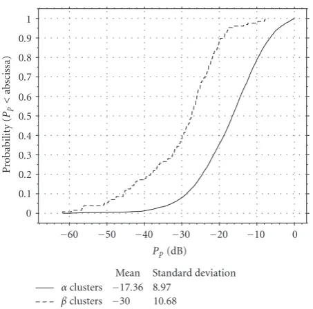
β-clusters resulted, where the distinctions between the two are as follows: (i) α-clusters were mainly a result of the mathematical/automatic clustering approach, whereas β -clusters were that of the manual clustering approach; (ii) manyα-clusters had overlapping clusters whereasβ-clusters had clear-cut delineation of their associated/corresponding scatterers, thus they have physical meaning; (iii)α-clusters had more energy than β-clusters. The results show that these overlapping clusters could basically be considered as outcomes of automatic clustering since they comprised the majority of the observed channel in terms of their power proportion. Furthermore, only a few clusters had a clear delineation of their dispersion. There is a difficulty then in judging the physical realism of overlapping clusters. This overlapping defeats the concept of spatial multiplexing, where cluster channel models that are used in simulations must be satisfactorily accurate. Moreover, this further points to a need for the physical interpretation and validation of clustering results, which is an initial step done in this paper, and further refinement or improvement is called for. This may somehow address the arbitrariness in identifying clusters. From these results, one may infer partial clustering of the channel at the MS. However, there is indeed a great deal
of arbitrariness in defining and determining clusters [7]. For example, the general consensus is that a cluster is a group of paths that have “similar” characteristics but is “distinct” from other path groups, but its quantification may differ from one automatic clustering to another (like the power-weighted multipath component distance [9]; cosine angle for directions and absolute delay difference [11]). Furthermore, from the systems-engineering view, cluster scatterers may not be important, which may be contrary to the radio-propagation-engineering view. Hence, the characteristics of these clusters are shown in what follows.
4.2. Cluster Scatterer Mechanism Classes. As discussed in
Section 3, propagation mechanism classes were taken from the results. Table 8 shows the cluster propagation mech-anism classes whereas Table 9 gives the type of scatterers corresponding to the clusters. Sinceβ-clusters had a clearer delineation thanα-clusters, only β-clusters are included in
Table 9.
As a comparison, in a similar area [45], the BS direction and facing BS direction were noted to have strong multipath contributions. For street directions, it has been observed that later-arriving multipaths propagate through street canyons [46], and in [47] it was observed that a significant number of multipaths comes from such directions. These observations are consistent with the values in Table 8, where the street direction dominated. In the same table, the BS direction and facing BS direction classes have almost the same contribution. Furthermore, the cluster scatterers were mostly metallic-type materials followed by concrete, asphalt, and brick, as shown inTable 9.
4.3. Cluster Characteristics. The condensed parameters of the cluster characteristics considered are the following:
(i) cluster average power (Pave)
(ii) number of clusters (iii) cluster fading factor (κ)
(iv) cluster delay
(v) cluster spreads (στ,σφ,σθ)
(vi) cluster polarization ratios.
The cluster fading factor is defined here as the ratio of the power of the strongest cluster to that of all the other clusters. It is pointed out thatσφ was computed according
Table10: Summary of cluster statistical parameters in urban/suburban macrocellular environments.
Cluster parameters
Kawasaki, Japan [this paper] Helsinki, Finland [6] Louvain-la-Neuve, Belgium [7]
Street residential-industrial Streetc Squarec Residential Campus Science park
(230–400 m)a (∼500 m)a (∼300 m)a (300–400 m)a (50–400 m)a (260–450 m)a
Meanb Stdevb Mean Stdev Mean Stdev Mean Stdev Mean Stdev Mean Stdev
Pave[dB] −15.35
−28.17 13.8311.24 − − − − −10.24d 5.18d −9.02d 5.6d −8.16d 5.72d
K 6.837.11 0.994.76 14 − 10 − 1.01 0.61 1.11 0.59 1.6 0.73 κ[dB] 4.261.43 5.245.33 3.65 2.29 2.26 1.99 −0.14 6.39 2.5 6.53 −1.4 6.54 τ[μs] 1.111.1 0.2710.255 2.83 1.04 1.38 0.46 0.22d 0.21d 0.19d 0.21d 0.13d 0.13d
σφAoD[◦] 4.671.34 5.551.25 − − − − − − − − − −
σφAoA[◦] 29.438.42 15.1820.8 4.2 1.94 4.57 2.07 11.09 2.04 9.18 2.13 11.74 1.89
σθAoD[◦] 2.831.17 3.861.25 − − − − − − − − − −
σθAoA[◦] 6.83.83 4.632.84 − − − − − − − − − −
στ[ns] 29.35
16.5 37.3223.9 27.22 40.68 28.5 42.57 10.46 1.78 8.28 1.88 9.1 1.78
XPR [dB]e − − 10.39 4.69 10.72 2.37 − − − − − −
XPRBS
V [dB] 8.63
8.73 5.25.37 − − − − − − − − − −
XPRBS
H[dB] 9.77
9.88 4.594.95 − − − − − − − − − −
XPRMSV [dB] 9.24
8.61 4.465.95 − − − − − − − − − −
XPRMS
H [dB] 9.15
10.01 4.955.87 − − − − − − − − − −
CPR [dB] −0.52−1.28 3.744.8 − − − − − − − − − −
aBS-MS distance. bα-clustersβ-clusters. csingle realization. d50th percentile data.
esingle-input multiple-output (SIMO).
ambiguous 2πperiodicity. The four cross-polarization ratios and co-polarization ratio of the clusters were computed, respectively, as follows:
XPRBSV =10 log10
⎛
⎝l∈CkγVV,l
2
l∈CkγVH,l 2
⎞
⎠, (18)
XPRBSH =10 log10 ⎛ ⎝
l∈CkγHH,l 2
l∈CkγHV,l 2
⎞
⎠, (19)
XPRMSV =10 log10
⎛
⎝l∈CkγVV,l
2
l∈CkγHV,l 2
⎞
⎠, (20)
XPRMSH =10 log10 ⎛ ⎝
l∈CkγHH,l 2
l∈CkγVH,l 2
⎞
⎠, (21)
CPR =10 log10
⎛ ⎝
l∈CkγVV,l 2
l∈CkγHH,l 2
⎞
⎠. (22)
The cross-polarization ratio (XPR) indicates the degree of polarization of the paths in a cluster incur from being vertically polarized to being horizontally polarized, or vice versa, whereas the copolarization ratio (CPR) shows the degree of vertical polarization with respect to the horizontal
polarization. In the notation in (18)–(21), XPRMSV , for example, is the XPR at the MS for paths that originated with V polarization, with the channel assumed to be reciprocal.
The mean and standard deviation of the cluster charac-teristics are placed together in Table 10. In the table, stdev refers to the standard deviation. The mean and standard deviation of the data in [6, 7] were also calculated and then tabulated. Observing this table, the angular spreads at the MS were larger than at the BS, indicating further that the degree of cluster scattering was concentrated at the MS. The σφAoA of the α-clusters was remarkable due to their overlapping characteristics. Compared to the COST 273 MIMO channel model [3], its corresponding
σφAoA is 35◦. Overall, the results are relatively comparable given the difference of the measured routes and setup. In addition, the results were influenced mostly by the different clustering criteria used by each author. These criteria basically give the cluster definition. It is also noted that the high delay resolution of the channel sounder that was used could include or exclude clusters that were subsequently identified by the methodology discussed inSection 3. Future target applications may have different capabilities (e.g., transmission scheme) and/or may not have such resolution in place in user terminals right away.
4.4. Parameter Correlation. To examine any linear
Power Number of clusters Fading factor Delay Delay spread Azimuth AoA spread Elevation AoA spread Azimuth AoD spread Elevation AoD spread XPRBS Number of clusters Fading factor Delay Delay spread Azimuth AoA spread Elevation AoA spread Azimuth AoD spread Elevation AoD spread XPRBS
(b)β-clusters
Figure8: Correlation coefficient matrix of the cluster parameters.
Table 11: Medium-to-large correlation among the α-cluster parameters.
Parameter 1 Parameter 2 Correlationcoefficient
Azimuth AoD spread Elevation AoD spread 0.86
Power Delay −0.58
Azimuth AoA spread Elevation AoA spread 0.56
Power Elevation AoD spread 0.52
Fading factor Elevation AoD spread 0.52
Fading factor Delay −0.47
Elevation AoA spread XPRBS
V −0.41
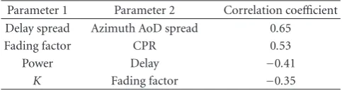
Table12: Medium-to-large correlation among theβ-cluster param-eters.
Parameter 1 Parameter 2 Correlation coefficient
Delay spread Azimuth AoD spread 0.65
Fading factor CPR 0.53
Power Delay −0.41
K Fading factor −0.35
medium-to-large correlation coefficients are tabulated in Tables 11 and 12. Not included in the table are those polarization parameters that correlated due to the reciprocity of the channel.
Considering the common results of both clusters, the correlation between cluster power and delay and also that of fading factor and delay are apparent, given that clusters with long delays have smaller power than those with short delays.
Forα-clusters in the considered macrocell, the azimuth and elevation AoD spread correlation could indicate that the spreading at the BS was concentrated toward the MS given that their spreads are also small as seen inTable 10. For the
azimuth and elevation AoA spread correlation, it could attest that the spreading becomes proportional to the scattering object. These two results may seem to be connected with the correlation between the elevation AoD spread and (i) the power, and also (ii) the fading factor, thus signifying the concentration of theseα-clusters. In the case of the elevation AoA spread and the XPRBSV correlation, it may roughly follow
that polarization rotation still occurs even when the cluster elevation dispersion is narrow.
For the β-clusters, the correlation between the delay spread and azimuth AoD spread corresponds to the majority of the propagation mechanism class. In the considered macrocell, the street direction is somehow concentric from the BS, which is lateral to where the MS is located (see
Figure 2). Thus a large cluster azimuth AoD spread corre-sponds to those multipaths that would incur more delays in going through those street canyons. This delay spread and angular spread correlation has also been observed in [49]. For the correlation between the fading factor and CPR, it could show that the dominant clusters were vertically polar-ized. Lastly, the negative correlation between the number of clusters and the fading factor could indicate that when there are more clusters in the scenario, the tendency of having dominant clusters is somehow dampened. These correlation results are consistent with the observed results previously discussed in this paper.
5. Conclusions
results were validated by identifying their corresponding or associated scatterers in the physical environment. Using this approach resulted in having (i) mathematical clusters, which are mostly characterized by overlapping clusters and are basically an outcome of automatic clustering, and (ii) small clusters, which have small power but clearly delineated clusters as produced by the manual clustering approach.
The overlapping of clusters makes it difficult to judge their physical realism, which further leads to the need for the physical interpretation of automatic clustering results, which is an initial step done in this paper and needs further improvement. This may somehow address the arbitrariness in identifying clusters. Due to the standoffpresent in defining clusters and their physical analysis, the authors proceeded to show the characteristics of both the mathematical clusters and small clusters. It was found that the street propagation mechanism class dominated. As a result of manual clustering, the physical realism of multipath clusters was also identified in terms of the type of the scatterer material. Metallic materials, followed by concrete, and then asphalt were the major types of cluster scatterers. It was found that the considered cluster characteristics agree with existing results, however, the difference largely depends on the criteria set forth by the clustering approach.
It is expected that the statistical property of the wireless channel will be different in other environments, for other frequency bands (e.g., 0.7, 30, and 60 GHz), and for other channel sounder resolutions. Secondary reasons for the differences are the modeling and various approaches used in the channel estimation and the subsequent channel analysis, synthesis, verification, errors, and application goals. With the use of the high-resolution channel sounder at 4.5 GHz in the urban macrocell considered here, it is noted that the target application and its available processing could define if the cluster characteristics in the evaluation would aid in its overall design. The disadvantages of the methodology are the expensive computation of simulated annealing in automatic clustering and the considerable user interaction required in the manual clustering approach. On the other hand, the automatic clustering results are better since they are not confined to local minima limitations, and the manual clustering approach could give an aspect of the physical scattering realism of the clusters, which is lacking in many automatic clustering results in the available litera-ture. Furthermore, this bicombinational clustering approach underscores the importance of incorporating validation in cluster identification. It is noted that further research work on improving the multipath clustering approach, as well as doing the channel analysis/modeling further is vital in order to understand the characteristics of multipath clusters.
Acknowledgment
The National Institute of Information and Communications Technology of Japan (NICT) is acknowledged for funding and supporting this research.
References
[1] M. Toeltsch, J. Laurila, K. Kalliola, A. F. Molisch, P. Vainikainen, and E. Bonek, “Statistical characterization of
urban spatial radio channels,”IEEE Journal on Selected Areas
in Communications, vol. 20, no. 3, pp. 539–549, 2002.
[2] H. Asplund, A. A. Glazunov, A. F. Molisch, K. I. Pedersen, and M. Steinbauer, “The COST 259 directional channel
model-part II: macrocells,” IEEE Transactions on Wireless
Communications, vol. 5, no. 12, pp. 3434–3450, 2006.
[3] L. Correia, Mobile Broadband Multimedia Networks:
Tech-niques, Models and Tools for 4G, Academic Press, Oxford, UK,
2006.
[4] J. Laurila, K. Kalliola, M. Toeltsch, K. Hugl, P. Vainikainen, and E. Bonek, “Wideband 3D characterization of mobile
radio channels in urban environment,”IEEE Transactions on
Antennas and Propagation, vol. 50, no. 2, pp. 233–243, 2002.
[5] K. Yu, Q. Li, and M. Ho, “Measurement investigation of tap
and cluster angular spreads at 5.2 GHz,”IEEE Transactions on
Antennas and Propagation, vol. 53, no. 7, pp. 2156–2160, 2005.
[6] L. Vuokko, P. Vainikainen, and J. Takada, “Clusters extracted from measured propagation channels in macrocellular
envi-ronments,”IEEE Transactions on Antennas and Propagation,
vol. 53, no. 12, pp. 4089–4098, 2005.
[7] C. Oestges and B. Clerckx, “Modeling outdoor macrocellular
clusters based on 1.9-GHz experimental data,”IEEE
Transac-tions on Vehicular Technology, vol. 56, no. 5, pp. 2821–2830,
2007.
[8] J. Salo, J. Salmi, N. Czink, and P. Vainikainen, “Automatic clustering of nonstationary MIMO channel parameter
esti-mates,” inProceedings of the 12th International Conference on
Telecommunications (ICT ’05), Cape Town, South Africa, May
2005.
[9] N. Czink, P. Cera, J. Salo, E. Bonek, J.-P. Nuutinen, and J. Ylitalo, “A framework for automatic clustering of parametric
MIMO channel data including path powers,” inProceedings of
the 64th IEEE Vehicular Technology Conference (VTC ’06), pp.
114–118, Montreal, Canada, September 2006.
[10] W. Dong, J. Zhang, X. Gao, P. Zhang, and Y. Wu, “Cluster identification and properties of outdoor wideband MIMO
channel,” inProceedings of the 66th IEEE Vehicular Technology
Conference (VTC ’07), pp. 829–833, Baltimore, Md, USA,
September-October 2007.
[11] M. Kwakkernaat and M. Herben, “Analysis of scattering in mobile radio channels based on clustered multipath
esti-mates,”International Journal of Wireless Information Networks,
vol. 15, no. 3-4, pp. 107–116, 2008. [12] http://www.channelsounder.de.
[13] M. Landmann, A. Richter, and R. Thoma, “Performance evaluation of antenna arrays for high-resolution DOA
estima-tion in channel sounding,” inProceedings of the International
Symposium on Antennas and Propagation (ISAP ’04), Sendai,
Japan, August 2004.
[14] M. Landmann, W. Kotterman, and R. Thoma, “On the influence of incomplete data models on estimated angular
distributions in channel characterisation,” inProceedings of
the 2nd European Conference on Antennas and Propagation
(EuCAP ’07), pp. 1–8, Edinburgh, UK, November 2007.
[15] R. Thoma, M. Landmann, and A. Richter, “RIMAX—a maximum likelihood framework for parameter estimation
the International Symposium on Antennas and Propagation
(ISAP ’04), pp. 53–56, Sendai, Japan, August 2004.
[16] A. Richter, Estimation of radio channel parameters: models
and algorithms, Ph.D. dissertation, Ilmenau University of
Technology, Ilmenau, Germany, 2005.
[17] M. Steinbauer, A. F. Molisch, and E. Bonek, “The
double-directional radio channel,” IEEE Antennas and Propagation
Magazine, vol. 43, no. 4, pp. 51–63, 2001.
[18] L. Materum, K. Sivasondhivat, J. Takada, I. Ida, and Y. Oishi, “Identification of relatively strong clusters in an NLOS scenario at a small urban macrocell mobile station,” in Proceedings of the International Symposium on Antennas and
Propagation (ISAP ’07), pp. 157–160, Niigata, Japan, August
2007.
[19] L. Materum, J. Takada, I. Ida, and Y. Oishi, “Improved multipath clustering of a small urban macrocellular MIMO
environment at 4.5 GHz,” inProceedings of the International
Symposium on Antennas and Propagation (ISAP ’08), pp. 854–
857, Taipei, Taiwan, October 2008.
[20] N. Czink and C. Oestges, “The COST 273 MIMO channel
model: three kinds of clusters,” inProceedings of the 10th IEEE
International Symposium on Spread Spectrum Techniques and
Applications (ISSSTA ’08), pp. 282–286, Bologna, Italy, August
2008.
[21] K. Sivasondhivat, J. Takada, I. Ida, and Y. Oishi, “Experimental analysis and site-specific modeling of channel parameters at
mobile station in an urban macrocellular environment,”IEICE
Transactions on Communications, vol. E91-B, no. 4, pp. 1132–
1144, 2008.
[22] J. MacQueen, “Some methods for classification and analysis
of multivariate observation,” inProceedings of the 5th Berkeley
Symposium on Mathematical Statistics and Probability, pp.
281–297, Berkeley, Calif, USA, December-January 1967. [23] W. H. E. Day, “Complexity theory: an introduction for
practitioners of classification,” inClustering and Classification,
P. Arabie, L. J. Hubert, and G. De Soete, Eds., pp. 199–233, World Scientific, London, UK, 1996.
[24] W. J. Welch, “Algorithmic complexity: three NP-hard
prob-lems in computational statistics,”Journal of Statistical
Com-putation and Simulation, vol. 15, no. 1, pp. 17–25, 1982.
[25] M. R. Garey and D. S. Johnson,Computers and Intractability: A
Guide to the Theory of NP-Completeness, W. H. Freeman, New
York, NY, USA, 1979.
[26] P. Brucker, “On the complexity of clustering problems,” in
Optimization and Operations Research, R. Henn, B. Korte, and
W. Oettli, Eds., vol. 157 ofLecture Notes in Economics and
Mathematical Systems, pp. 45–54, Springer, Berlin, Germany,
1978.
[27] I. S. Dhillon, Y. Guan, and B. Kulis, “Weighted graph cuts
with-out eigenvectors a multilevel approach,”IEEE Transactions on
Pattern Analysis and Machine Intelligence, vol. 29, no. 11, pp.
1944–1957, 2007.
[28] H. Frigui and R. Krishnapuram, “A robust competitive clustering algorithm with applications in computer vision,”
IEEE Transactions on Pattern Analysis and Machine Intelligence,
vol. 21, no. 5, pp. 450–465, 1999.
[29] D. J. C. MacKay,Information Theory, Inference and Learning
Algorithms, Cambridge University Press, New York, NY, USA,
2003.
[30] S. Kirkpatrick, C. D. Gelatt Jr., and M. P. Vecchi,
“Optimiza-tion by simulated annealing,”Science, vol. 220, no. 4598, pp.
671–680, 1983.
[31] N. Metropolis, A. W. Rosenbluth, M. N. Rosenbluth, A. H. Teller, and E. Teller, “Equation of state calculations by fast
computing machines,”The Journal of Chemical Physics, vol. 21,
no. 6, pp. 1087–1092, 1953.
[32] W. K. Hastings, “Monte Carlo sampling methods using
Markov chains and their applications,”Biometrika, vol. 57, no.
1, pp. 97–109, 1970.
[33] V. Murino, A. Trucco, and C. S. Regazzoni, “Synthesis
of unequally spaced arrays by simulated annealing,” IEEE
Transactions on Signal Processing, vol. 44, no. 1, pp. 119–122,
1996.
[34] E. Aarts and J. Korst, Simulated Annealing and Boltzmann
Machines, John Wiley & Sons, New York, NY, USA, 1989.
[35] N. Czink, R. Tian, S. Wyne, et al., “Tracking time-variant cluster parameters in MIMO channel measurements,” in Proceedings of the 2nd International Conference on
Communi-cations and Networking in China (CHINACOM ’07), pp. 1147–
1151, Shanghai, China, August 2007.
[36] N. Czink, E. Bonek, L. Hentil¨a, J.-P. Nuutinen, and J. Ylitalo, “Cluster-based MIMO channel model parameters extracted
from indoor time-variant measurements,” in Proceedings
of IEEE Global Telecommunications Conference
(GLOBE-COM ’06), pp. 1–5, San Francisco, Calif, USA,
November-December 2006.
[37] P. J. Rousseeuw, “Silhouettes: a graphical aid to the
interpre-tation and validation of cluster analysis,”Journal of
Computa-tional and Applied Mathematics, vol. 20, no. 1, pp. 53–65, 1987.
[38] D. L. Davies and D. W. Bouldin, “A cluster separation
measure,”IEEE Transactions on Pattern Analysis and Machine
Intelligence, vol. 1, no. 2, pp. 224–227, 1979.
[39] T. Cali ´nski and J. Harabasz, “A dendrite method for cluster
analysis,”Communications in Statistics: Theory and Methods,
vol. 3, no. 1, pp. 1–27, 1974.
[40] D.-J. Kim, Y.-W. Park, and D.-J. Park, “A novel validity index
for determination of the optimal number of clusters,”IEICE
Transactions on Information and Systems, vol. E84-D, no. 2, pp.
281–285, 2001.
[41] A.-O. Boudraa, “Dynamic estimation of number of clusters in
data sets,”Electronics Letters, vol. 35, no. 19, pp. 1606–1608,
1999.
[42] N. Bolshakova and F. Azuaje, “Improving expression data
mining through cluster validation,” inProceedings of the 4th
International IEEE EMBS Special Topic Conference on
Informa-tion Technology ApplicaInforma-tions in Biomedicine (ITAB ’03), pp. 19–
22, Birmingham, UK, April 2003.
[43] A. Hinneburg, Density-based clustering in large databases
using projections and visualizations, Ph.D. dissertation, Martin
Luther University of Halle-Wittenberg, Halle, Germany, 2002.
[44] N. Czink, The random-cluster model—a stochastic MIMO
channel model for broadband wireless communication systems
of the 3rd generation and beyond, Ph.D. dissertation, Vienna
University of Technology, Vienna, Austria, 2007.
[45] N. Kita, W. Yamada, A. Ando, D. Mori, T. Takao, and H. Watanabe, “Characteristics of direction of arrival in residential
area in 5-GHz band,” in Proceedings of the IEICE Society
Conference, vol. B-1–14, Hokkaido, Japan, September 2005.
[46] A. Molisch, Wireless Communications, Wiley-IEEE Press,
Chichester, UK, 2005.
[48] European Telecommunications Standards Institute, “Uni-versal mobile telecommunications system (UMTS); spacial channel model for multiple input multiple output (MIMO)
simulations,”ETSI TR-125-996-V7.0.0, 2007.
[49] N. Czink, E. Bonek, L. Hentil¨a, P. Ky¨osti, J.-P. Nuutinen, and J. Ylitalo, “The interdependence of cluster parameters in
MIMO channel modeling,” inProceedings of the 1st European
Conference on Antennas and Propagation (EuCAP ’06), pp. 1–6,