R E S E A R C H
Open Access
Landweber iterative regularization
method for identifying the unknown source
of the time-fractional diffusion equation
Fan Yang
*, Xiao Liu, Xiao-Xiao Li and Cheng-Ye Ma
*Correspondence: [email protected] School of Science, Lanzhou University of Technology, Lanzhou, Gansu 730050, P.R. China
Abstract
In this paper, we investigate an inverse problem to determine an unknown source term that has a separable-variable form in the time-fractional diffusion equation, whereby the data is obtained at a certain time. This problem is ill-posed, and we use the Landweber iterative regularization method to solve this inverse source problem. Two kinds of convergence rates are obtained by using an a priori and an a posteriori regularization parameters choice rules, respectively. Numerical examples are provided to show the effectiveness of the proposed method.
MSC: 65M30; 35R25; 35R30
Keywords: time-fractional diffusion equation; ill-posed problem; unknown source; Landweber iterative method
1 Introduction
In recent years, diffusion equations with fractional-order derivatives play an important role in modeling contaminant diffusion processes. A fractional diffusion equation mainly describes anomalous diffusion phenomena because fractional-order derivatives enable the description of memory and hereditary properties of heterogeneous substances []. Replac-ing the standard time derivative with a time fractional derivative leads to the time frac-tional diffusion equation, and it can be used to describe superdiffusion and subddiffusion phenomena [–]. In some practical problems, the diffusion coefficients, a part of bound-ary data, initial data, or source term may be unknown. We need additional measurement to identify them, which leads to some fractional diffusion inverse problem. Nowadays there are many research results about fractional diffusion inverse problem. In [], the authors considered an inverse problem of recovering boundary functions from transient data at an interior point in a -D semiinfinite half-order time-fractional diffusion equation. In [], the authors applied a quasi-reversibility regularization method to solve a backward problem for the time-fractional diffusion equation. In [–], the authors studied an in-verse problem in a spatial fractional diffusion equation by using the quasi-boundary value method and truncation method. In [, ], the authors determined the unknown source in one-dimensional and two-dimensional fractional diffusion equations. In [], the au-thors used the dynamic spectral method to consider the inverse heat conduction problem of a fractional heat diffusion equation in -D setting. In [], the authors used an optimal
regularization method to consider the inverse heat conduction problem of a fractional heat diffusion equation. In [, ], the authors used the quasi-reversibility regularization method and Fourier regularization method to identify the unknown source for a fractional heat diffusion equation.
In this paper, we investigate an inverse problem for the time-fractional diffusion equa-tion with variable coefficients in a general bounded domain[, ]:
⎧
() and is a symmetric uniformly elliptic operator:
Lu(x) =
where the coefficient functionsaijandc(x) satisfy
aij=aji, ν
As in [], define the Hilbert space
D (–L)p= [,T] and is known. The space-dependent source termf(x) is unknown. We use the data
u(x,T) =g(x) to determinef(x). The noise datagδ∈L() satisfies
gδ–gL()≤δ, (.)
where · denotes theL() norm, andδ> is a noise level.
convergence rate for the a priori parameter choice method isO(δ), and for the a posteri-ori parameter choice method, it isO(δ). In [], the authors used the Tikhonov regular-ization method to solve problem (.), but the error estimates between the regularregular-ization solution and the exact solution also have the saturation phenomenon under the two pa-rameter choice rules. In this study, we use the Landweber iterative regularization method to solve this problem. Our error estimates under two parameter choice rules have no sat-uration phenomenon, and the convergence rates are allO(δpp+).
This paper is organized as follows. Section presents the Landweber iterative regular-ization method. Section presents the convergence estimates under a priori and a poste-riori choice rules. Section presents some numerical examples to show the effectiveness of our method. Section presents a simple conclusion.
2 Landweber iterative regularization method In this section, we first give some useful lemmas.
Lemma .([]) Forη> and <α≤,we have≤Eα,(–η) < ,and Eα,(–η)is
com-pletely monotonic,that is,
(–)n d
n
dηnEα,(–η)≥, ∀n∈N∪ {}. (.)
Lemma .([]) Forβ∈Randα> ,we have
Eα,β(z) =zEα,α+β(z) +
(β), z∈C. (.)
Lemma .([]) For <α< ,λ> ,and q∈C(,T),we have
Dα
t
t
q(τ)(t–τ)α–Eα,α –λ(t–τ)α
dτ
=q(t) –λ
t
q(τ)(t–τ)α–Eα,α –λ(t–τ)α
dτ. (.)
Moreover,ifλ= ,then
Dαt
t
q(τ)(t–τ)α–dτ=(α)q(t), <t≤T.
Lemma . ([]) For anyλnsatisfyingλn≥λ> ,there exists a positive constant C
depending onα,T,λsuch that
C
Tαλ
n
≤Eα,α+ –λnTα
≤
Tαλ
n
. (.)
Lemma . For any <x< ,we have
x<√x (.)
and
Due to Lemma ., using the separation of variables, we obtain the solution of problem (.)
u(x,t) = ∞
n=
fn
t
q(τ)(t–τ)α–Eα,α –λn(t–τ)α
dτ
Xn(x), (.)
whereλnare the eigenvalues of the operator –L, and the corresponding eigenfunctions
areXn(x),fn= (f(x),Xn(x)). Usingu(x,T) =g(x), we have
g(x) = ∞
n=
fn
T
q(τ)(T–τ)α–Eα,α –λn(T–τ)α
dτ
Xn(x), (.)
wheregn= (g(x),Xn(x)). Since –Lis a symmetric uniformly elliptic operator, we get []
<λ≤λ≤ · · · ≤λn≤ · · ·, lim
n→∞λn= +∞. (.)
Lethn(T) :=
T
q(τ)(T–τ)α–Eα,α(–λn(T–τ)α)dτ.
So we obtain
gn=fnhn(T). (.)
Then
fn=
gn
hn(T)
, (.)
that is,
f(x) = ∞
n=
fnXn(x) =
∞
n=
gn
hn(T)
Xn(x). (.)
We only need to solve the following first kind integral equation to obtainf(x):
(Kf)(x) =
k(x,ξ)f(ξ)dξ=g(x), x∈, (.)
where the kernel is
k(x,ξ) = ∞
n=
hn(T)Xn(x)Xn(ξ).
Fork(x,ξ) =k(ξ,x),K is a self-adjoint operator. Iff ∈L(), theng∈H() from []. BecauseH() is compactly embedded inL(), we have thatK:L()→L() is a compact operator. So problem (.) is ill-posed []. Assume thatf(x) has the following a priori bound:
f(x)
D((–L)
p
)≤E, p> , (.)
Theorem .([]) Let q(t)∈C[,T]satisfy q(t)≥q> for all t∈[,T],and let f(x)∈
D((–L)–p)satisfy the a priori bound condition f(·)
D((–L)–
p
)≤E, p> .
Then we have
f(·)≤CE
p+g(x)
p
p+, (.)
where C:= (Cq)–
p p+.
Now we use the Landweber iterative method to obtain the regularization solution for (.) and rewrite the equationKf =gin the formf = (I–aK∗K)f +aK∗gfor somea> . Iterate this equation:
f,δ(x) := , fm,δ(x) = I–aK∗Kfm–,δ(x) +aK∗gδ(x), m= , , , . . . ,
wheremis an iterative step number, and the selected regularization parameterais called the relaxation factor and satisfies <a<K. SinceKis a self-adjoint operator, we obtain
fm,δ(x) =a
m
k=
I–aK∗Kk–Kgδ(x). (.)
We get
fm,δ(x) =Rmgδ(x) =
∞
n=
– ( –ahn(T))m
hn(T)
gnδXn(x), (.)
wheregδ
n= (gδ,Xn(x)).
3 Error estimate under two parameter choice rules
In this section, we give two convergence estimates under an a priori regularization param-eter choice rule and an a posteriori regularization paramparam-eter choice rule, respectively.
3.1 An a priori regularization parameter choice rule
Theorem . Let f(x)be the exact solution of problem(.),and let fm,δ(x)be the
regular-ization Landweber iterative approximation solution.Choosing the regularization param-eter m= [r],where
r=
E δ
p+
, (.)
we have the following convergence rate estimate:
fm,δ(·) –f(·)≤CE
p+δ
p
p+, (.)
where[r]denotes the largest integer less than or equal to r,and C=√a+ (
aC q
p )
–p is a
Proof By the triangle inequality we have
fm,δ(·) –f(·)≤fm,δ(·) –fm(·)+fm(·) –f(·). (.)
We first give an estimate for the first term. From conditions (.) and (.) we have
fm,δ(·) –fm(·)=
Using Lemma . and Theorem ., we have
Letλn:=tand
F(t) :=
–aqC
t m
t–p. (.)
LettsatisfyF(t) = . Then we easily get
t=
aq
C(m+p)
p
> . (.)
Thus
F(t) =
– p m+p
m
aqC(m+p)
p
–p
,
that is,
F(t)≤
aq C
p
–p
(m+ )–p. (.)
Thus we obtain
Q(n)≤
aqC p
–p
(m+ )–p. (.)
Hence
fm(·) –f(·)≤
aqC p
–p
(m+ )–pE. (.)
Combining (.) and (.) and choosing the regularization parameterm= [r], we get
fm,δ(·) –f(·)≤CE
p+δ
p
p+, (.)
whereC:= √
a+ (aq C
p )
–p.
We complete the proof of Theorem ..
3.2 An a posteriori regularization parameter choice rule
We consider the a posteriori regularization parameter choice in the Morozov discrepancy and construct regularization solution sequencesfm,δ(x) by the Landweber iterative reg-ularization method. Letτ > be a given fixed constant. Stop the algorithm at the first occurrence ofm=m(δ)∈Nwith
Kfm,δ(·) –gδ(·)≤τ δ, (.)
wheregδ ≥τ δis constant.
(b) limm→+∞γ(m) =gδ; (c) limm→γ(m) = ;
(d) γ(m)is a continuous function.
Lemma . For fixedτ> ,combining Landweber’s iteration method with stopping rule
(.),we obtain that the regularization parameter m=m(δ,gδ)∈N
Proof From (.) we get the representation
Rmg=
On the other hand, it is easy to see thatmis the minimum value and satisfies
KRmgδ–gδ=Kfm,δ–gδ≤τ δ.
Hence
KRm–g–g ≥KRm–gδ–gδ–(KRm––I)g–gδ ≥τ δ–KRm––Iδ
≥(τ– )δ.
On the other hand, using (.), we obtain
so that
(τ– )δ≤S(n)E. (.)
Using Lemma ., we have
S(n)≤ –aqTαEα,α+ –λnTα
Combining (.) with (.), we obtain
m≤
The proof of lemma is completed.
Theorem . Let f(x)be the exact solution of problem(.),and let fm,δ(x)be the
Proof Using the triangle inequality, we obtain
fm,δ(·) –fm(·)≤fm,δ(·) –fm(·)+fm(·) –f(·). (.)
Applying (.) and Lemma ., we get
fm,δ(·) –fm(·)≤√amδ≤CE
p+δ
p
p+, (.)
whereC= (qp+ C)
(q
τ–)
p+.
For the second part of the right side of (.), we get
K fm(·) –f(·)= ∞
n=
– –ahn(T)mgnXn(x)
= ∞
n=
– –ahn(T)m gn–gnδ
Xn(x)
+ ∞
n=
– –ahn(T)mgnδXn(x).
Combining (.) and (.), we have
K fm(·) –f(·)≤(τ+ )δ. (.)
Using Theorem . and (.), we have
fm(·) –f(·)
D((–L)
p
)= ∞
n=
– –ahn(T)mfnλpn
≤E.
So
fm(·) –f(·)≤C
(τ+ )
p p+Ep+δ
p
p+. (.)
Hence
fm,δ(·) –f(·)≤ C(τ+ )
p p++C
Ep+δ
p
p+. (.)
The theorem is proved.
4 Numerical implementation and numerical examples
In this section, we provide numerical examples to illustrate the usefulness of the proposed method. Since analytic solution of problem (.) is difficult, we first solve the forward prob-lem to obtain the final datag(x) using the finite difference method. For details of the fi-nite difference method, we refer to [–]. Assume that= (, ) and taket=TN and
and the grid points in the space interval [, ] arexi=ix,i= , , , . . . ,M. Noise data are
generated by adding random perturbation, that is,
gδ(x) =g(x) +g(x)ε· rand size(g)– ,
whereεreflects the noise level. The total error levelgcan be given as follows:
δ=gδ–g=
M+
M+
i=
gi–giδ
.
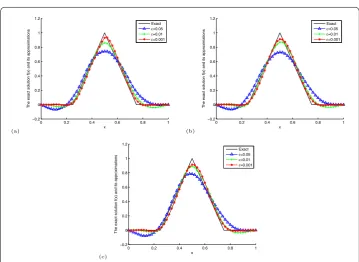
In our numerical experiments, we takeT= . When computing the Mittag-Leffler func-tion, we need a better algorithm in []. In applications, the a priori boundEis difficult to obtain, and thus we only give the numerical results under the a posteriori parameter choice rule. In the following three examples, the regularization parameter is given by (.) with
τ = .. To avoid the ‘inverse crime,’ we use a finer grid to computer the forward problem, that is, we takeM= ,N= and chooseM= ,N= for solving the regularized inverse problem. In the computational procedure, we leta(x) =x+ ,c(x) = –(x+ ), and the time-dependent source termq(t) =e–t.
Example Take functionf(x) = [x( –x)]αsinπx.
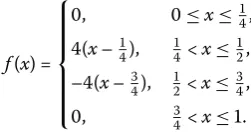
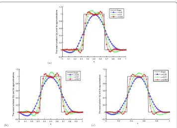
Example Consider the following piecewise smooth function:
f(x) = ⎧ ⎪ ⎪ ⎪ ⎪ ⎪ ⎨ ⎪ ⎪ ⎪ ⎪ ⎪ ⎩
, ≤x≤, (x–), <x≤, –(x–), <x≤, , <x≤.
(.)
Example Consider the following initial function:
f(x) = ⎧ ⎪ ⎪ ⎨ ⎪ ⎪ ⎩
, ≤x≤, , <x≤, , <x≤.
(.)
Figure 1 The exact and regularized terms given by the a posteriori parameter choice rule for Example 1: (a)α= 0.2, (b)α= 0.5, (c)α= 0.9.
Figure 3 The exact and regularized terms given by the a posteriori parameter choice rule for Example 3: (a)α= 0.2, (b)α= 0.5, (c)α= 0.9.
Table 1 The posteriori regularization parametermunder differentαandεfor Example 1
ε= 0.05 ε= 0.01 ε= 0.001
α= 0.2 1,359,781 7,324,093 72,760,970
α= 0.5 1,073,344 5,810,540 58,185,563
α= 0.9 1,033,583 5,622,036 51,073,803
Table 2 The posteriori regularization parametermunder differentαandεfor Example 2
ε= 0.05 ε= 0.01 ε= 0.001
α= 0.2 87,014 454,794 4,115,710
α= 0.5 86,575 420,586 4,073,802
α= 0.9 79,713 411,222 4,314,369
Table 3 The posteriori regularization parametermunder differentαandεfor Example 3
ε= 0.05 ε= 0.01 ε= 0.001
α= 0.2 91,970 416,913 4,747,577
α= 0.5 92,115 447,945 4,337,702
α= 0.9 87,505 415,486 4,309,392
5 Conclusion
and the convergence rates are allO(δ p
p+) under two parameter choice rules. Meanwhile,
numerical examples verify that the Landweber iterative regularization method is efficient and accurate. In the future work, we will continue to study some source terms that depend on both time and space variables.
Acknowledgements
The authors would like to thank the editor and referees for their valuable comments and suggestions that improved the quality of our paper. The work is supported by the National Natural Science Foundation of China (11561045, 11501272) and the Doctor Fund of Lan Zhou University of Technology.
Competing interests
The authors declare that they have no competing interests.
Authors’ contributions
The main idea of this paper was proposed by FY, and XL prepared the initial manuscript and performed all the steps of the proofs in this research. All authors read and approved the final manuscript.
Publisher’s Note
Springer Nature remains neutral with regard to jurisdictional claims in published maps and institutional affiliations.
Received: 10 July 2017 Accepted: 10 November 2017
References
1. Berkowitz, B, Scher, H, Silliman, SE: Anomalous transport in laboratory-scale, heterogenous porous media. Water Resour. Res.36(1), 149-158 (2000)
2. Metzler, R, Klafter, J: Subdiffusive transport close to thermal equilibrium: from the Langevin equation to fractional diffusion. Phys. Rev. E61(6), 6308-6311 (2000)
3. Scalas, E, Gorenflo, R, Mainardi, F: Fractional calculus and continuous-time finance. Phys. A284, 367-384 (2000) 4. Sokolov, IM, Klafter, J: From diffusion to anomalous diffusion: a century after Einstein’s Brownian motion. Chaos15,
1-7 (2005)
5. Bhrawy, AH, Baleanu, D: A spectral Legendre-Gauss-Lobatto collocation method for a space-fractional advection diffusion equations with variable coefficients. Rep. Math. Phys.72(2), 219-233 (2013)
6. Fairouz, T, Mustafa, I, Zeliha, SK, Dumitru, B: Solutions of the time fractional reaction-diffusion equations with residual power series method. Adv. Mech. Eng.8(10), 1-10 (2016)
7. Gómez-Aguilar, JF, Miranda-Hernández, M, López-López, MG, Alvarado-Martinez, VM, Baleanu, D: Modeling and simulation of the fractional space-time diffusion equation. Commun. Nonlinear Sci. Numer. Simul.30(1), 115-127 (2016)
8. Benson, DA, Wheatcraft, SW, Meerschaert, MM: Application of a fractional advection-dispersion equation. Water Resour. Res.36(6), 1403-1412 (2000)
9. Sun, HG, Zhang, Y, Chen, W, Donald, MR: Use of a variable-index fractional-derivative model to capture transient dispersion in heterogeneous media. J. Contam. Hydrol.157, 47-58 (2014)
10. Zhang, Y, Sun, HG, Lu, BQ, Rhiannon, G, Roseanna, MN: Identify source location and release time for pollutants undergoing super-diffusion and decay: parameter analysis and model evaluation. Adv. Water Resour.107, 517-524 (2017)
11. Murio, DA: Stable numerical solution of fractional-diffusion inverse heat conduction problem. Comput. Math. Appl.
53(1), 492-501 (2007)
12. Liu, JJ, Yamamoto, M: A backward problem for the time-fractional diffusion equation. Appl. Anal.80(11), 1769-1788 (2010)
13. Wei, T, Wang, J: A modified quasi-boundary value method for an inverse source problem of the time-fractional diffusion equation. Appl. Numer. Math.78, 95-111 (2014)
14. Wang, JG, Zhou, YB, Wei, T: Two regularization methods to identify a space-depend source for the time-fractional diffusion equation. Appl. Numer. Math.68, 39-75 (2013)
15. Zhang, ZQ, Wei, T: Identifying an unknown source in time-fractional diffusion equation by a truncation method. Appl. Math. Comput.219(11), 5972-5983 (2013)
16. Kirane, M, Malik, AS: Determination of an unknown source term and the temperature distribution for the linear heat equation involving fractional derivative in time. Appl. Math. Comput.218(1), 163-170 (2011)
17. Kirane, M, Malik, AS, Al-Gwaiz, MA: An inverse source problem for a two dimensional time fractional diffusion equation with nonlocal boundary conditions. Math. Methods Appl. Sci.36(9), 1056-1069 (2013)
18. Xiong, XT, Zhou, Q, Hon, YC: An inverse problem for fractional diffusion equation in 2-dimensional case: stability analysis and regularization. J. Math. Anal. Appl.393, 185-199 (2012)
19. Xiong, XT, Guo, HB, Liu, XH: An inverse problem for a fractional diffusion equation. J. Comput. Appl. Math.236, 4474-4484 (2012)
20. Yang, F, Fu, CL: The quasi-reversibility regularization method for identifying the unknown source for time fractional diffusion equation. Appl. Math. Model.39, 1500-1512 (2015)
21. Yang, F, Fu, CL, Li, XX: The inverse source problem for time fractional diffusion equation: stability analysis and regularization. Inverse Probl. Sci. Eng.23(6), 969-996 (2015)
23. Pollard, H: The completely monotonic character of the Mittag-Leffler functionEα(–x). Bull. Am. Math. Soc.54,
1115-1116 (1948)
24. Kilbas, AA, Srivastava, HM, Trujillo, JJ: Theory and Applications of Fractional Differential Equations. North-Holland Mathematics Studies, vol. 204. Elsevier, Amsterdam (2006)
25. Sakamoto, K, Yamamoto, M: Initial value/boundary value problems for fractional diffusion-wave equations and applications to some inverse. J. Math. Anal. Appl.382(1), 426-447 (2011)
26. Kirsch, A: An Introduction to the Mathematical Theory of Inverse Problems. Springer, New York (1996)
27. Murio, DA: Implicit finite difference approximation for the time-fractional diffusion equation. Comput. Math. Appl.
56(4), 1138-1145 (2008)
28. Yang, M, Liu, JJ: Implicit difference approximation for the time-fractional diffusion equation. J. Appl. Math. Comput.
22(3), 87-99 (2006)
29. Podlubny, I, Kacenak, M: Mittag-Leffler function, The MATLAB routine (2006). http://www.mathworks.com/ matlabcentral/fileexchage