ABSTRACT
BHANDARI, LAKSHAY RAKESHKUMAR. Navigation of Autonomous Differential Drive Robot using End-to-End Learning. (Under the direction of Edward Grant).
Autonomous driving is and has been one of the most prevailing robotics research topics
in recent years. Having said that, it draws attention that self driving vehicles demand a
tremendous amount of research from a variety of topics in engineering, mathematics and
science. Challenges remain in the fields of perception, localization and control. A basic
per-ception application that uses a camera feed requires an exhaustive pipeline which includes
data acquisition, image processing for feature extraction followed by the application of an
estimation model from classical machine learning, or deep learning, to identify objects in
the image using extracted features. Following the feature extraction phase, an algorithm for
object localization within the scene is applied; in order to generate instantaneous motion
control.
The research here follows on from research originally conducted by NVIDIA into
end-to-end learning for autonomous vehicles. The goal of the research here is focused on the
reduction of the pipeline size and on the effort required to implement multiple algorithms
for a range of tasks, e.g., tasks including feature extraction, object detection and object
localization, for an autonomous driving Wheelchair. Using just RGB images as the primary
perception input signal, the developed system generates instantaneous driving commands
for this Wheelchair.
Experiments with the above approach, embedded within a single trained Convolutional
Neural Network, can handle an entire perception pipeline and thereby reduce the burden
© Copyright 2019 by Lakshay Rakeshkumar Bhandari
Navigation of Autonomous Differential Drive Robot using End-to-End Learning
by
Lakshay Rakeshkumar Bhandari
A thesis submitted to the Graduate Faculty of North Carolina State University
in partial fulfillment of the requirements for the Degree of
Master of Science
Electrical Engineering
Raleigh, North Carolina
2019
APPROVED BY:
Andrew Rindos John Muth
Edward Grant
DEDICATION
To mumma, papa and my sisters who have been tremendously instrumental in my journey
BIOGRAPHY
The author hails from Surat, a city in Gujarat, India. Prior to joining the ECE graduate
program at NC State University, he worked as a Controls Engineer at Reliance Industries
Limited, India, following the completion of his Bachelor of Technology in Instrumentation
ACKNOWLEDGEMENTS
The work performed in this thesis over the course of two semesters has been possible due
to the indispensable support provided by my advisor, Dr. Edward Grant for fuelling my
enthusiasm in research in a highly budding and interesting field. All my learning in the
duration of this thesis has greatly consolidated my understanding of the concepts employed
in this work. My senior colleague, Hamed Mohammadbagherpoor has been very generous
and kind throughout, helping me whenever I was stuck at any stage.
My fellow researcher, Abhayjeet Singh Juneja, has been my companion in the endeavour
since the time we started working on the Wheelchair and experimenting with it for
integra-tion of AI into the navigaintegra-tion control system. We have spent innumerable hours developing
the system that was used in this work, learning a lot from each other. I would also like to
thank Dr. Andrew Rindos and Dr. John Muth for being members of my committee. I am
grateful to the people who have extended their help to collect hours worth of training data.
I can recall making them stand or walk in front of the wheelchair while I would operate the
wheelchair.
In addition, I cannot thank enough the people outside my academic bubble who have
motivated me to work hard each day. My mother, who has been always there to push me
and channelize my passion in right directions. My father and my sisters, for their constant
love and guidance. I am also grateful to my friends and roommates, who have helped me in
my hard times, both in academics and my personal life. All the support has made me feel
at home and made my passion in engineering and science even stronger and fuelled my
TABLE OF CONTENTS
LIST OF TABLES . . . vii
LIST OF FIGURES. . . viii
Chapter 1 INTRODUCTION. . . 1
1.1 Thesis statement . . . 3
1.2 Contributions . . . 3
1.3 Organization . . . 5
Chapter 2 BACKGROUND . . . 6
2.1 A Self-Driving Application . . . 7
2.1.1 Perception . . . 8
2.1.2 Localization . . . 17
2.1.3 Path Planning and Control . . . 19
Chapter 3 RELATED WORK AND MOTIVATION . . . 21
3.1 End-to-End Learning by NVIDIA . . . 21
3.2 Precursor to this Work . . . 24
3.2.1 Overview of the Test-Bench . . . 24
3.2.2 AUTONOMOUS NAVIGATION . . . 25
3.2.3 CHOICE OF PERCEPTION SENSOR FOR END-TO-END LEARNING 33 Chapter 4 SYSTEM DEVELOPMENT AND HYPOTHESIS. . . 35
4.1 Sensors: Perception . . . 38
4.1.1 Kinect . . . 38
4.1.2 Webcam . . . 38
4.2 Software and Hardware Architecture . . . 40
4.2.1 ROS Architecture . . . 42
4.2.2 Hardware pipeline . . . 44
4.3 The CNN . . . 45
4.3.1 Network Architecture . . . 45
4.3.2 Data Collection and Training . . . 45
4.3.3 Experimentation . . . 47
4.4 Motion Control . . . 49
4.5 TussleNet : Not a Net . . . 50
Chapter 5 EVALUATION . . . 52
Chapter 6 CONCLUSION . . . 61
Chapter 7 FUTURE SCOPE . . . 63
7.1 Using RNN . . . 64
7.2 Integration with IoT . . . 64
LIST OF TABLES
LIST OF FIGURES
Figure 3.1 Structure of Kinect node in ROS . . . 25
Figure 3.2 Object Detection in RGB image and corresponding Depth image . . . 28
Figure 3.3 Error calculation for Depth Precision Control . . . 30
Figure 3.4 Orientation of LiDAR sensor on Wheelchair (Top View) . . . 30
Figure 3.5 ROS node for LiDAR and Proximity Mapping algorithm . . . 33
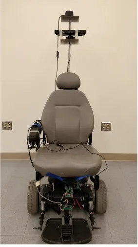
Figure 4.1 Wheelchair system . . . 37
Figure 4.2 Installation of webcam on Wheelchair . . . 39
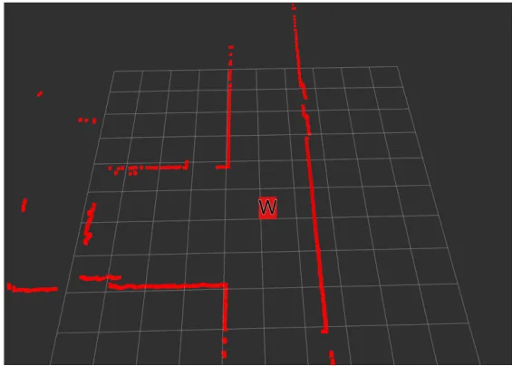
Figure 4.3 LiDAR scan of environment same as captured in Fig. 4.4 . . . 40
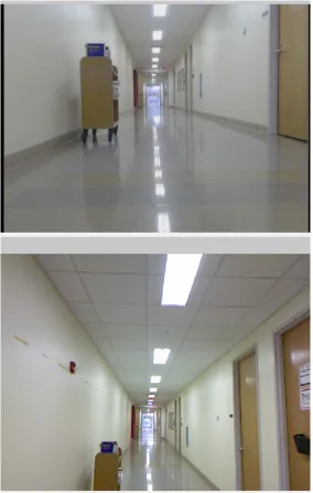
Figure 4.4 (From top) Webcam capture, Kinect capture . . . 41
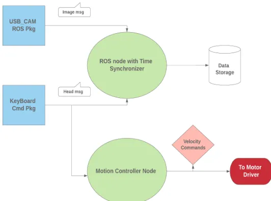
Figure 4.5 ROS architecture for training the CNN . . . 43
Figure 4.6 ROS architecture in deployed system . . . 44
Figure 4.7 Hardware pipeline . . . 45
Figure 4.8 CNN architecture for Regression Model . . . 48
Figure 5.1 Summary for trained model . . . 54
Figure 5.3 Performance scenario 2 . . . 54
Figure 5.2 Performance scenario 1 . . . 55
Figure 5.4 Performance scenario 3 . . . 55
Figure 5.5 Performance scenario 4 . . . 56
Figure 5.6 Performance scenario 5 . . . 56
Figure 5.7 A feature map in the middle of CNN . . . 57
Figure 5.8 Feature maps following conv2_2d layer (indoor) . . . 58
Figure 5.9 Feature maps following conv2_2d layer (outdoor) . . . 59
Figure 5.10 Feature maps following conv5_2d layer . . . 59
CHAPTER
1
INTRODUCTION
The rise of Artificial Intelligence in recent years has fulled various innovations in the fields
which have rather proved highly useful in human assistance in as simple tasks as reading
to as complex as driving. With the powerful hardware available to cater to the ever growing
computational needs of state of the art AI like Computer Vision, Autonomous Driving has
become one of the most sought after and researched topics, resulting in unprecedented
advancements in the field. It is expected that by the year 2020, the number of self-driving
cars on US roads will sore to as high as 10 million. In addition, with the advent of Internet of
Things, the number of connected smart vehicles is expected to grow to 250 million [Woo18].
the technology primarily aims to eradicate traffic incidents which are caused due to reasons
like distraction of the drivers while driving. In 2016, 84% of the car crashes recorded within
the US were rooted in distracted drivers. Other major contributor to car crashes found was
impaired drivers[Sta18], [Dav15]. Self-driving cars hold the potential to reduce the number
of accidents. On the contrary, it cannot be stated that with today’s self-driving technology
the accidents can be absolutely avoided. There have been cases which have put a halt to
deployment of self-driving cars on the road [The18], [Gri18].
Despite a few setbacks, there are a number of companies which are working to develop
state of the art technologies which can aid the self-driving cars [Fri17], both including
start-ups [Dix18]and well established giants [CBI18].
There are a number of steps involved for a single decision to be made by the autonomous
vehicle on the road which involve data acquisition and processing, perception, localization
and motion planning. Perception is usually done using sensors like Cameras, LiDARs,
Ultra-sonic, Radars either individually or with their signals fused together. With cameras, where
the principal signal is an image, a typical pipeline involves image processing, classification
techniques, object detection and localization within the scene and generating a control
action (instantaneous velocity or driving angle). This type of an approach, which is often
used for self-driving applications (e.g., HoG feature generation for detecting pedestrians
using Support Vector Machines [DT05a], obstacle detection in an image using a Neural
Network [How17]followed by bounding box estimation for each detected obstacle [Liu16a],
[RF17a], e.t.c.) not only pushes hardware in the heavy lifting region, but also increases the
complexity of the system with multiple algorithms to be interfaced with one another.
In this work, an approach previously used by NVIDIA [Boj16]is extended to autonomous
driving for Differential Wheel Drive robots in an indoor environment, with further
system can generate either of instantaneous velocity for robot wheels or driving angle
(angle with respect to the instantaneous motion) in contrast with the model proposed by
NVIDIA where motion prediction is given in the form of the turning radius. Furthermore,
an interactive pipeline is created which allows the user to take control in cases where the
autonomous mode reflects inaccurate predictions. As a result, it could be seen the
perfor-mance in the indoor environment was comparable with the previous implementation for
self-driving cars on the roads. Also, it could be inferred that the outcome could be achieved
with comparable performance with predictions being in the form of instantaneous velocity
and driving angles. Furthermore, generating driving angle predictions gives the liberty to
use system with regression or discrete output meaning either of a regression model or a
classification model can be used.
1.1
Thesis statement
"Current trends in perception for autonomous differential wheel drive robots use a complex
pipeline for navigation in the indoor environment, which can be simplified by leveraging
the end-to-end approach to encompass the system into a single neural network."
1.2
Contributions
This thesis delves in a unique approach for navigation for the robots involving differential
drive instead of a steering wheel as in cars. It aims to reduce the pipeline size and complexity
by mainly avoiding the need for different algorithms for obstacle detection and localization.
It is noted that the neural network used for object detection or classification can be modified
can be modified to map the input image to driving commands instead of detecting the
presence of an object or type of an object. Furthermore, the need to use an additional
algorithm to find the location of the detected objects in the image can be prevented as
well. Since the proposed system produces motion prediction based on the input scene
image, detection of objects and their location is done inherently and thus using the obstacle
detection or classification becomes redundant.
This work makes the following contributions:
• It is seen that the system developed for the differential drive robots for the
environ-ment with stated approach yields comparable results to the previous impleenviron-mentation
for self-driving cars on roads [Boj16].
• We modify the system to produce the motion prediction based on the input image as
either driving angles or instantaneous velocity directly. With output as the
instanta-neous velocity, the need to convert driving directions to velocity is also avoided.
• A separate pipeline is then built to train the neural network on the data where the
predictions are inaccurate. This can help the user to train the network while in
au-tonomous mode. We call this idea, rather than the CNN itself, the TussleNet as it aims
to capture the tussle between the user and the CNN.
As stated above, this is not the first work in the field that uses this approach for
au-tonomous driving application. We experiment with this tried approach to extend its
ap-plication in the indoor environment and differential drive robots. Previous notable works
have been published in the similar light in the past stressing on the end-to-end approach
1.3
Organization
The remainder of this thesis is structured as follows.
Chapter 2 provides a background on the technologies used in this work, and explains
a general pipeline used by many of the autonomous driving applications, especially in
the perception system. Chapter 3 provides the previous iteration of this work, along with
the other relevant work which have used a similar approach. In Chapter 4, we provide our
approach on the perception for autonomous differential drive robots. The hypothesis is
explained by providing a use case for a Wheelchair system which serves as a test bench
for this work. In Chapter 5 we summarize the performance evaluation of the system and
explain how the this approach can be used to reduce the size of perception pipeline. Finally,
in chapter 6, we conclude this work, and briefly touching upon its future scope in chapter
CHAPTER
2
BACKGROUND
This chapter will define a general methodology that can be used in any self-driving
applica-tion, be it for autonomous cars or differential drive robots; such as a wheelchair. Building
on that, the algorithms involved, such as for obstacle detection and localization, will be
explored in detail using classical machine learning techniques and also the more recent and
powerful deep learning techniques. There will be exploration into how these components
can be integrated to build a self-driving application. In addition, semantic segmentation
will be explored, as will instance segmentation and other benchmark works which laid
the foundation for computer vision techniques. These approaches contribute hugely to
2.1
A Self-Driving Application
Self-driving technology is already functioning and still evolving and showing improved
performance over previous iterations. As self-driving cars are meant to imitate human
behaviour, any such application is composed broadly on the following components:
• Data Acquisition and Processing: this includes sensors information being received by
the system and the processing of the information in order to be understood by the
algorithms downstream. This part may or may not involve sensor fusion.
• Perception: this includes building a map of the surroundings based on data provided
by various sensors such as cameras, LiDAR, ultra sonic, etc. either individually or
fused together.
• Localization: this involves making an estimate of the vehicle’s location withing the
environment [Cad16].
• Path Planning and Control: this includes making an estimate of the trajectory of the
vehicle based on the current sensor readings [Pad16].
At any sampling instant, the input signal, e.g., an image, 2-D or 3-D point cloud, has to
pass through a variety processing stages before motion can be predicted. This is followed by
signal processing which aims to remove noise and extract any useful information, e.g., a low
pass filter is used to retain the dc component of a signal and filter out the high frequency
noise. Specific applications involve image processing to remove noise from blurred images
or removing outliers from a 3-D LiDAR point cloud using a RANSAC algorithm [FB81].
The perception system, with the help of processed data from sensors, builds a virtual
required by the decision making algorithms further downstream in the process. Localization
can also be considered a part of the perception system; because it deals with the vehicles
environment as projected by the sensor data. A localization algorithm estimates the vehicle’s
position and pose with respect the the map/road. This can further aid in any motion
planning decisions. Since this work focuses on motion control using perception, the work
done on perception will be discussed in greater detail.
2.1.1
Perception
The perception system is the fundamental component in a self-driving application. It
pro-vides essential information about, or representation of, the environment. Such information
is required in order to estimate the motion at the current state and, in some cases, it can be
used to predict the motion at near future states. There are a number of sensors which can
be used for perception systems, including: (1) light detection and ranging (LiDAR) sensors,
(2) cameras and (3) radio detection and ranging (RADAR) sensors. A common shortcoming
of any perception systems is their need for clean, noiseless data. In addition, in situations
where computational resources are limited, data has to be compressed in order to process
it in an orderly fashion.
2.1.1.1 LiDAR
LiDAR is one of the most prevailing sensors being used in the autonomous driving industry.
LiDAR works by throwing out a large number of light pulses into the environment around
the vehicle, it then captures its representation using the reflected pulses. The representation
can be either 2-D or 3-D, depending on the LiDAR sensor used. It is quite accurate when
most of the available commercial LiDAR sensors are expensive. The major problem posed
by a LiDAR point cloud is its sparsity. With more erratic surroundings, a LiDAR point cloud
can become extremely complex. Also, LiDAR data cannot be compressed, on account that
it is already providing limited available information, e.g., x,y,z coordinates of an obstacle.
Hence, storing data with LiDAR can be memory expensive. As mentioned in [Pen17], there
are broadly three ways to process LiDAR data:
• Point cloud based - which uses the raw sensor data. With a finer representation, this
approach is expensive in terms of memory and processing time. Voxel based methods
are used as improvisations to this approach [Szé10], [PL17]
• Feature based - extracting features from the LiDAR point cloud helps in dealing with
data that prominently represents the key points from the environment which can aid
the decision making. [Wan11], [Yu05],[Alh02]
• Grid based - converting the LiDAR point cloud into several grids using an adaptive
discretization method as in [Vo15]has been shown to be successful and more memory
efficient.
In addition, for LiDAR sensors with less data points per sampling such as in a 2-D
LiDAR, median filter can be used to efficiently create a point cloud ready for decision
making algorithms. Median filters not only work for LiDAR point clouds, but can also be
used to remove noise from images. Median filters remove noise but leave intrinsic data
intact. Because of its wide reach of applications, there are many toolboxes which provide
inbuilt functions to perform median filtering. Due to the availability of a 2-D LiDAR, a
median filter was used to denoise the point cloud in previous iteration of this work as well.
Post processing the LiDAR data, perception becomes a two fold process, which involves
needed. The former component of the pipeline is referred to as clustering (or segmentation)
while the latter is called detection.
• Segmentation- it means clustering the data at point level or region level from the
point cloud into discrete groups with each group representing a feature, object, etc.
Some published works in this field revolve around edge based, region based, feature
based, model based or graph based segmentation algorithms.
– Edgebased techniques can be applied in scenarios where there are inherent
features available, such as edges (e.g., intersections and curbs on roads, door
frames indoors). Although approaches presented in work well, this represents a
very small subset of the environmental features a robot or an autonomous car
can deal with.
– Regionbased approaches move a step ahead and cluster the points based on a
common criterion such as Euclidean distance or surface normals. As opposed to
edge based approaches, region based approaches take into account the
neigh-borhood, i.e., some key points, making edge based approaches more general
purpose.
– Modelbased segmentation eradicates the need of finding seed points in the
Li-DAR point cloud as an improvement over region based methods. Also, as region
based approaches are dependent on the seed points alone for their accuracy,
fail-ing to select optimum key points may result in poor segmentation. Model based
algorithms utilize the mathematical models lying behind attributes like planes or
surfaces, shapes like spheres or cones, etc. The segmentation algorithm works by
clustering the points according to a particular parameter (e.g., points satisfying
following using this method are RANSAC (Random Sample Consensus) and HT
(Hough Transform). RANSAC has been also used for removing outliers from 3-D
point clouds by fitting a model. Many works, including [Sch07], [LK13]show
the successful use of RANSAC algorithm. Due to its efficiency, it has also been
adopted by popular libraries for point cloud processing such as [RC11]. HT is the
other extensively used algorithm using model based segmentation, as reviewed
in [Pen17]. Work states in [Vos04]shows detection of planar surfaces in 3-D
point clouds using vector normal to the surfaces. In [KM12], the HT is used to
detect cylinders in the 3-D point cloud generated by LiDAR.
– Attributebased segmentation tries to capture the underlying attributes in the
point cloud which are not replicated wholly by the spatial information alone.
The success of the attribute based approach is shown in [YD13]where difficult
objects like poles have been identified from within a point cloud.
– Graphbased methods are powerful pertaining to their node-edge structure
which can easily and efficiently represent an environment. Not only the
rep-resentation is apt, using graph based structures also makes it easy to apply
graph theory which has proven to be powerful in many domains such as
im-age segmentation, localization and many more. In [Te18], the authors propose
segmentation of point cloud using regularized graph CNN approach that
ex-ploits spectral graph theory and treats features in points as signals on the graph.
Delving on similar lines, several approaches like k-nearest neighbours [GF09]
have been used for segmentation of point cloud. In addition, as mentioned in
[Pen17], graph based structures have been very useful in fusing multiple sensors’
Apart from the above mentioned approaches, many machine learning architectures
have been used to find the features from within the 3-D point cloud. While new works
in the field focus on deep learning [Qi17], [Te18], [Rus08], the older works have also
shown how classical machine learning can be utilized for segmentation [GF09].
• Detection- Post segmentation, all the clusters need to be categorized into different
objects, such as road curbs, poles, walls, pedestrians, e.t.c. In[Moo09], ground clusters
using histogram over normal to the surfaces. Other work was shown in [Zha13]which
could also classify segments above the ground such as vegetation, building and
pedestrians. The authors in [Yan18]propose a computationally efficient approach
using a bird eye view of the environment instead and applying a 3-D CNN on the
point cloud to detect objects pertaining to self-driving scenarios. In [Li17]however,
another fully connected 3-D CNN is used to detect vehicles. The reason behind such
a huge number of works using deep learning is the availability of labelled data-sets.
KITTI data-set [Gei13]is one of the most extensively used data-sets for training the
neural networks for object detection in point clouds. The cons of using deep learning
networks however include computational complexity and memory usage. The work in
[Rie17]introduces a more memory efficient Octree Network which greatly increases
the input cluster resolutions.
2.1.1.2 Computer Vision and Camera
While LiDAR throws light to generate the point cloud from the objects in the environment,
a camera can be used to produce either RGB (Red Blue Green) images or depth image. The
VIS (visible) cameras can capture the scene by discretizing the visible spectrum into R, G
VIS cameras, with knowledge of focal distance, can be used to perform stereoscopy vision,
also called stereo vision. Cameras which also provide the depth information are also called
RGBD cameras, due to an addition channel (for RGB and Depth).
Detecting objects in 2-D images has mainly been the task of machine learning
tech-niques. With RGB images, machine learning has been one of the most used approaches
to detect and classify objects in the scene. Machine learning approaches used until early
2000s involve classical machine learning architectures such as Support Vector Machines
(SVM), Random Forest Classifiers, e.t.c. Later approaches involving deep networks can
in-herently extract features alongside the detection. Deep learning networks used extensively
in the field of computer vision are MLP (Multi Layer Perceptrons) and (CNN) Convolutional
Neural Networks. In context of self-driving, RNN (Recurrent Neural Networks) have also
been used. In this section, we will discuss the approaches which involve classical machine
learning architectures and deep neural networks.
• Classical Machine Learning and Feature extraction
SVM [CV95], Random Forest Classifier [Ho95]are some of the very powerful
architec-tures which have been used for the purpose of identifying objects and classification
in images. Although they have been known to solve some of the most challenging
problems in computer vision, they are not equipped to handle images directly at
the input. Instead, the images are needed to be processed to extract useful features
prior to inputting to any of these architectures. Rooting for this, image processing is a
separate area of research which aims at feature extraction from the images. We will
discuss the features relevant to the domain of self-driving which have been developed
to aid computer vision with such learning methods.
pertaining, but not limited to road lanes, pedestrians, road signs, traffic signals, e.t.c.
There have been developed a number of tools for operating on images with different
kind of filters (or kernels) to extract features and form feature descriptors (or vectors)
which may represent key parameters and their location within the images. Various
tried and tested filter kernels include mean filters, median filters, Gaussian smoothing,
etc. Other types of filter kernels find the edges (vertical and horizontal or tilted), and
can detect surfaces. The author in [Lab06]talks about detecting lanes on the roads,
while outperforming previous works which would generate inaccurate results due to
factors like shadows on the roads. As seen in survey [Pen17], lane feature extraction
can be done by using edge detection [Ned04; Li03]and color [TETT09; Sun06a].
These feature vectors can be passed through SVM [Zha05], Random Forest Classifiers
[Cho12; Xia16], or other boosted or ensemble learning methods [Bah10]to indicate
the presence (or absence) of lanes [Gop12].
Other objects of interest are road signs. Work in [MB07]uses SVM for the task. Also, it
is safe to mention that most of the road signs have fixed shapes (e.g., circles, triangles)
and hence it would make much sense to fit such possible shapes in the image to a
model and using HT [Bal81], and matching the identified shapes with signs available
in the database using feature matching techniques like SIFT and SURF [Pan13], which
are also often used in the process of localization.
Traffic lights are also one of the static objects which need to be identified by the
perception systems for driver assistance. [DCN09]shows a work in this domain.
Again, HT is used in [OO09]for feature extraction for traffic lights, while [Liu02]uses
genetic algorithm with search region limits on the image to do the same.
Major breakthrough in pedestrian detection is HOG (Histogram of Oriented
Gradi-ents) feature descriptor [DT05b]. In this work, gradient is calculated at pixel level to
generate feature vectors for edges which could represent human bodies. SVM is used
to classify images as containing humans or not. In [Sun06b]Gabor filter is used to
generate Gabor feature descriptor for detecting rear view vehicles. In [Wen15], the
authors develop a efficient method to select Haar-like [VJ01]features using AdaBoost
[Sch13]with sample’s feature and its corresponding label.
• Deep Learning
Deep learning has been one of the most researched topics for long time now because
of its powerful capabilities in solving challenges in computer vision. One of the
greatest wins for deep networks such as Convolutional Neural Networks (CNN) is
their inherent feature extraction. A CNN has the capability to take a 3-D (RGB) image
as its input as opposed to its classical machine learning equivalents, such as SVM.
Machine learning is used to make informed decisions based on its learning from the
training data provided. So in order to train a system, we need to parse the data and
then pass it through the system, and comparing its output with the training labels
to generate a loss metric. Deep learning does exactly the same, except it does not
always require data parsing explicitly. A CNN comprises of Convolution filters which
perform image processing implicitly, without having the need to have an additional
image processing algorithm. The features being extracted from an image will be
hidden from the user and will highly depend on the training labels provided in the
training data. The authors in [Sza05]describe the use of CNN with automatic feature
pedestrians. Similarly in [Fuk15], CNN is used for the same task while comparing it to
different networks for the task of pedestrian detection. While pedestrian detection is
an example, networks such as MLP and CNN can detect and classify multiple number
of objects in an image if provided with good training data.
Classification tasks have been made extremely powerful with great works in the filed.
With ILSVRC (ImageNet Large Scale Visual Recognition Challenge), many researchers
have come together to out do previous works in object detection and classification.
LeNet [LeC98], AlexNet [Kri12], VGGNet [SZ14], GoogLeNet [Sze15], ResNet [He16]
are some of the great works which won the challenge with astonishing results in
classification tasks. Following these benchmarks, many researchers have published
their own modified version of the networks developed previously. The availability of
diverse data-sets such as [Eve10], [Lin14]and [Den09]has greatly fuelled the success
of these works.
In context of self-driving vehicles, object detection and localization within the image
is also needed in order to make motion planning decisions. Usual approaches used
in the field are creating bounding boxes around the detected objects in the image.
One of the very first networks, R-CNN was presented in [Uij13], with multiple small
CNN models to explore the features in sub-areas (Region of Interest) of the image
and passing them through SVMs for classification purposes. An improvement over
this work is Fast R-CNN, presented in [Gir15]where a single CNN was used over
the image instead of multiple CNNs over multiple Regions of Interest. Yet again,
the system was improved with Faster R-CNN presented in [Ren15], where a RPN
(Region Proposal Network) is used to select RoIs instead of selecting multiple RoIs
Fully Connected Network) is used where the ResNet-101 is used to detect feasible
areas in the image where objects are most likely present. All the above networks for
object detection have worked well, but were not ready for deployment in real-time. A
great work which worked in real-time was YOLO (You Only Look Once) [Red16]. Its
improvised version, Fast YOLO [Sha17]showed great performance at 155 FPS (Frames
Per Second). Another recent development is shown in SSD (Single Shot Detector)
[Liu16b], which used the data-set to decide an initial guess for selecting RoIs. This
approach is better as it eliminates the need of looking for RoIs from scratch. Even
better versions of YOLO, YOLOv2 [Zha17]and YOLO9000 [RF17b]have outperformed
all the networks with their high FPS and accuracy.
Another class of methods used for perception is image segmentation. It refers to
pixel-wise classification where each pixel is classified according to the object or type
of object it constitutes. [KU19]talks about various works which have been used for
image segmentation for self-driving application. Image segmentation can help the
perception system lay down pixel-wise labelling of lanes, vehicles, pedestrians, trees,
e.t.c. present on the road. The results can then be used to perform motion planning.
2.1.2
Localization
Localization is the process of estimating the position of a robot in an environment. In
addition to perception, a robot’s location is required to plan a path between a source and
destination. In order to reach a destination, the autonomous system needs to know where it
currently is to predict the subsequent states of motion. There are various sensors involved
in autonomous driving which can help the system with estimating the location. These
• Odemetry sensors - IMU (Inertial Measurement Unit) measures the net acceleration
of the robot in real world coordinates (x,y,z). The velocity and displacement from the
starting point of the robot can then be derived by single and double time
integra-tion, respectively. Wheel encoders can sense the velocity of the wheels and has the
capability of tracking the location with respect to starting point. In such techniques,
where displacement of robot is measured using wheel displacement over time, the
estimated location can be highly inaccurate due to drift in sensor readings. Kalman
filter [WB95]is a recursive technique which can be used to give better estimates of
the location as time evolves, reducing the uncertainty of estimation. It can also be
used to fuse the data from two different sensors (e.g., IMU and Encoder) to get an
even better estimate, where uncertainty of measurement of both sensors is included.
• Perception sensors - Camera, LiDAR, RADAR, e.t.c are sensors which can help the
system figure out the location of the robot using the features such as landmarks in
the environment. Particle filter [DM96]is a special type of Bayesian filter which use
the observations of these sensors (e.g., an instantaneous or continuous LiDAR scan,
an image or group of frames, e.t.c) and use existing maps to find out the location.
In many cases, especially in case of on-road vehicles, GPS (Global Positioning System)
provides with a map of the environment, except in tough places like tunnels and
under-ground roads. To tackle this, IMU mounted GPS systems have been introduced.
Apart from these situations, GPS is not expected to work in indoor environments (e.g.,
buildings). In this case, either a map can be built in advance, or on the fly as the robot moves
and discovers the indoor environment. Rooted in solving this problem, SLAM (Simultaneous
Localization And Mapping) has become a popular research area in recent years. Many SLAM
A survey in [Bre17]states the types of SLAM as Filter based (application of Bayesian filters
such as Kalman, Particle filters), Optimization based (uses Bundle Adjustment as a loss
function to compare sensor readings and the map). Some of the notable filter based SLAM
are EKF-SLAM [Bai06]and particle filter based [ED06]. Using BA (Bundle Adjustment),
ORB-SLAM [MA15]and ORB-SLAM2 [MAT17]have been very successful. Other works such
as [Tat17]employ deep learning to learn the mapping of a monocular image to the depth
image associated with it to perform SLAM.
2.1.3
Path Planning and Control
Path planning and control is the final step in the pipeline as it is responsible for the final
control action - the velocity of wheels to control the direction of motion. After the map
has been constructed, its graph representation can be used to apply various algorithms for
path planning. These algorithms work by establishing node-node connections in graph
structures. Some of popular algorithms used for path planning are A* [Del09], RRT (Rapidly
exploring Random Trees), RRT* , PRM (Probabilistic RoadMap) [KF11]. PRM can lay down
the free route for a robot in the configurations space, while A*, RRT and RRT* can plan the
path dynamically at each state of the robot’s motion.
Following path planning, a control action needs to be generated. The control action
may vary depending on the type of robot, here, we will talk about differential drive robots.
In this case, the control action is generating wheel velocities such that the robot attains a
particular velocity and moves in the planned direction. This final task can be considered
as dead reckoning, where the control actions for next state are generated with respect to
the previous state of the robot, and the knowledge of the map. For instance, in a previous
CHAPTER
3
RELATED WORK AND MOTIVATION
The research reported on here was motivated by the work of NVIDIA and the early work
done on this project. The idea for this work comes from [Boj16]. The former shows the
implementation for an on-road self-driving car, the latter is a set of experiments using
sensors other than LiDAR to enable autonomous navigation in indoor environments.
3.1
End-to-End Learning by NVIDIA
The work in [Boj16]leverages the pattern recognition capabilities of a CNN architecture,
features learned are highly dependent on the data examples provided. Hence, it is possible
to regulate this aspect of a CNN, to have it use relevant data according to the application
being built. The authors in this work develop DAVE-2 system inspired by DAVE (DARPA
Autonomous Vehicle) developed in [LeC04]. The AI architecture used in this work also
shares the essence of the work in [Pom89]which used a dense neural network for
self-driving application.
The DAVE-2 system uses the CAN (Controller Area Network) of the vehicle to collect
vehicle’s steering angle, provided by the user, in association with the time-stamped video
stream. Therefore, the data-set for training the CNN consists of frames and driving
com-mands as its output. The authors mention that to make their system independent of the
geometry of the vehicle, they are using the inverse of the turning radius 1r, whereris the
turning radius, as the driving command. Therefore, the training data-set contains a number
of frames, each with a corresponding inverse of turning radius. In addition, the authors
use three cameras, one camera on either side of the vehicle, and a camera in the center. All
cameras face forward. This camera configuration can accommodate any off-center shifts
in image data and it allows the system to learn recovery in case of disturbances. These
off-center shifts are also applied to the corresponding steering commands to ensure for
robust training.
Data collection was conducted in a variety of environments and in a variety of lighting
conditions. This introduced variance into the training data-set. Since the system is
end-to-end, it was important for the network to see a variety of scenarios; in order to understand
tasks in all environments, in settings ranging from a bright sunny day to a gloomy evening.
Data was collected in scenarios where the drivers were following lanes, changing lanes and
turning. The data pertaining to lane following was retained while the rest of the data was
the end-to-end approach. Also, the video stream was sampled at 10 FPS to avoid having too
similar consecutive frames (and steering angles). Since there is a bias with respect to driving
straight on the roads, a big proportion of data retained contained roads with curving lanes.
The CNN architecture proposed was adopted, although with some modifications in the
work pertaining to this thesis. These alterations will be explained in the later sections.
For testing the trained CNN, a simulation was designed; one where the performance of
the system could be evaluated. The performance metric, apart from the testing the losses
of the CNN, was the duration of the experimental cycle when no human intervention was
needed. The pipeline developed in the simulation or testing phases proved capable of
handling human intervention, but does not take account of human intervention during
the system’s training cycle. Another important aspect of the simulation pipeline is the
manner in which it deals with image transformation, i.e., how it account’s for the vehicle
moving away from it’s ground truth, which essentially helps assessing the system in case of
disturbances. Based on their assumption that human drivers need 6 seconds for adjusting
a vehicle after disturbance on the road, the authors came up with an equation for the
autonomy
Au t o n o m y =1−6.IN TE
(3.1)
whereIN is the number of interventions by human driver in order to correct the system
inTE seconds of autonomous driving mode.
Finally, the "mysterious" working of the CNN was also observed. As can be seen in
[Boj16], the internal states of the CNN clearly extract features like lanes and lane curvature,
without explicitly extracting such features at the beginning. The authors also mention that
extraction.
3.2
Precursor to this Work
The work in this thesis builds on previous works into autonomous wheelchair research at
NC State. A similar task of autonomous navigation was achieved using the usual pipeline
involving perception, object classification, object detection and planning for motion
con-trol of an autonomous robot. The test bench used for experimentation is a Jazzy Select
Wheelchair [Pri19]. .
3.2.1
Overview of the Test-Bench
The wheelchair is powered using DC motors, which are run by 2 series connected 12V
batteries. In order to develop autonomous navigation system on the wheelchair, it was
equipped with a variety of perception sensors (kinect camera [Mic18]and RPLIDAR-A1/A3
[Sla18]), development boards including Raspberry Pi and Arduino Uno, and a motor driver
. Since the power supply for most of the development boards is less than 24V, power
converters were used to regulate the power supply as needed.
The structure of the wheelchair was modified to house the LiDAR and Kinect camera
at locations which could be useful during perception. The LiDAR used was a 2-D scanner,
which proved sufficient for operating in static surroundings; like building corridors and
doorways, while the Kinect camera proved helpful for detecting objects in front of the
wheelchair, both dynamic and static, like dustbins, pedestrians, e.t.c. LiDAR and kinect are
connected serially to a GPU enabled laptop, which also runs the middleware ROS (Robot
Operating System) [Qui09]master. Computationally intensive algorithms run on a PC
as the Raspberry Pi. ROS envelopes the entire system with different modules (and nodes,
written in both Python and C++). Running the system on ROS is advantageous as it enables
to synchronize data inflow and control signal outflow.
3.2.2
AUTONOMOUS NAVIGATION
Kinect and LiDAR data was interpreted separately, with their individually developed
al-gorithms, to control the motion of the wheelchair. Pipelines for both these sensors were
different, but with the common goal of sending velocity commands to the DC motors
through the motor driver for controlling the motion of the wheelchair. The velocity
com-mands were generated so as to achieve an instantaneous turning angle, based on the
perceived environment.
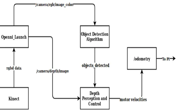
3.2.2.1 Object Detection and Obstacle Avoidance
The Kinect is RGBD camera. In addition to monochrome images, can also capture a
depth map of the scene being viewed. For obstacle avoidance using a Kinect, both the
monochrome image and the depth image are used. Readily available ROS packages like
Openni_Launch enables both images to be used. Using the ROS CvBridge package, Kinect
images are converted into a format which can be processed by OPENCV, an open source
li-brary available to work with images and computer vision. Also, the images can be subscribed
to by different nodes within ROS on respective topics, i.e., as ROS messages. In this pipeline,
two nodes working simultaneously subscribe to RGB and depth images respectively. The
application of both images is described below.
• Object Detection- For object detection, RGB images were used. Here, the research
published in [How17]along with the research in [Liu16a]were used. The former is
a light-weight CNN architecture based on depth-wise separable convolutions. The
performance of depth-wise separable convolution is shown to be N1 +Dk12 times faster
than regular convolution filters, whereNis the number of filters in the layer andDk
is the dimension of the filter kernel. The MAP (Mean Average Precision) of MobileNet
is evaluated at 88.7% on COCO data-set. Based on this performance, a decision was
made to use MobileNet as the base network. In this research MobileNet runs below
the SSD object detection algorithm.
The SSD architecture builds upon the base CNN used, but it ignores the fully
con-nected layers attached to the end of the CNN. These fully concon-nected layers are
re-placed with extra convolution layers, which extract useful features at different scales
and sizes. These features are then utilized for detecting multiple objects. Similar to
the difference between ground truth bounding boxes and the predicted locations
of bounding boxes. They also used this technique to estimate the confidence loss. A
key feature of SSD is that it avoids the need to propose all the bounding boxes from
scratch. The network learns from the data-set the most probable object locations
within an image. This helps network speed and increases its efficiency. The bounding
boxes that are estimated in advance are called priors.
Using a combination of SSD and MobileNet, the developed system can efficiently
classify and detect objects within the scene from RGB images.
• Depth Perception and Control- There are multiple ways to estimate the distance of
an object (represented by a pixel or a set of pixels) from a camera. One of the ways is
using an available pin-hole camera model along with a calibration matrix. With this
approach depth information can be estimated from an RGB image. The second, and
more convenient way, is to use depth information directly if it is available. With the
wheelchair, the Kinect camera provides the depth information directly. The depth
image computed from the RGB image, which was passed through the MobileNet+
SSD pipeline, was used to estimate the distance from the camera to objects (and
hence from the wheelchair).
The node working on RGB images published a custom message contains the
infor-mation regarding the bounding boxes (object locations and their sizes). A separate
node, which used the depth image from the Kinect camera, subscribed to this custom
message and projects the locations of the bounding boxes onto the depth image.
The region on the depth image which was occupied by the bounding boxes in the
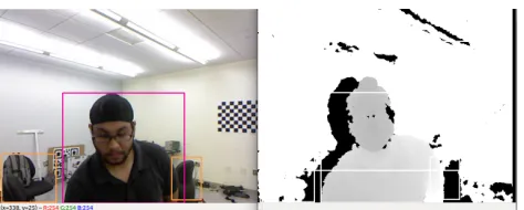
corresponding RGB image was considered for checking the depth value. A threshold
Figure 3.2Object Detection in RGB image and corresponding Depth image
speed. Hence, the depth image was continually checking for any object(s) being closer
than 2.5 meters. Object(s), if found to be closer than 2.5 meters, were avoided.
In order to control wheelchair motion during obstacle avoidance, a proportional
con-troller only was added to the system initially. In order for the proportional concon-troller
to work an error signal was generated.
Obstacle avoidance works by removing the closest object from a specific region (called
a safe zone) of the camera frame, which eventually leads to planning the path around
the detected object. The safe zone is defined as a region in pixel space where no
object should exist. Only then is there a safe passage of the wheelchair. Obstacles are
prioritized based on the following:
– Obstacles in safe zone and closer than 2.5 meters - Highest Priority
– Obstacles in safe zone and farther than 2.5 meters - Medium Priority
– Obstacles not in safe zone - Zero Priority
Because the control algorithm is based on Proportional control only, error is defined
by how much of a detected obstacle is inside the safe zone. Examples of obstacles in
a depth image safe zone are shown in Fig.3.3. The center of the obstacle is calculated.
If an obstacle in the left side of the safe zone, relatively, then the error is calculated as
in an image in the right side of the safe zone, this gives a relative negative error. The
equations (3.3a) and (3.3b) represent the calculated velocity of the right and left
motors of the wheelchair based on error.
e =o b s t a c l e_r i g h te d g e −s a f e_z o n e_l e f te d g e (3.2a) e =o b s t a c l e_l e f te d g e−s a f e_z o n e_r i g h te d g e (3.2b)
vr= (vr e f −kp∗e)∗v e lf l a g (3.3a) vl = (vr e f +kp∗e)∗v e lf l a g (3.3b) wherekpis the proportional gain,eis the error calculated (in pixels) from depth image,
vr e f is the set speed for wheelchair,vr andvl are the speeds calculated for right and
left motors respectively, andv e lf l a g is the fail safe variable to bring the wheelchair
to a complete halt. A positive errore (or obstacle on left) makes the wheelchair turn
right and a negative errore (or obstacle on right) makes the wheelchair turn left.
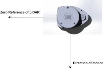
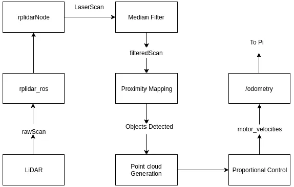
3.2.2.2 PROXIMITY MAPPING WITH LIDAR
For this application, a 2D LiDAR was used. The top view of the LiDAR with respect to the
wheelchair is shown in Fig.3.4. The direction of motion of the wheelchair aligns with a
LiDAR scan data at 90◦. A ROS compatible library for LiDAR called "rplidar" was used to
interpret and communicate LiDAR scan data between different nodes. The package comes
with a node for LiDAR which converts the raw LiDAR scan data to ROS messages. This
Figure 3.3Error calculation for Depth Precision Control
resolution of 1◦in a 2D plane. Based on the orientation, the field of view for this application
lies between 0◦and 180◦. A point cloud was generated at each sampling instant, but only for
objects which lie inside the wheelchair’s previously defined threshold distance, i.e, 2.5m.
• Pre-processing of LiDAR Scan Data- With the help of the rplidar ROS package, a
laser scan is received with values of distance between objects and LiDAR in the range
0◦to 360◦. The received values are not immune to noise, which calls for the need to
pre-process the data before it is used for mapping the surroundings, and eventually
in the control algorithm. In the pre-processing algorithm, a median filter is used to
remove noise from the scanned data. The implementation of this filter can be seen in
(3.4). After applying this filter to the raw scan data provided by the ROS node, an array
of 360 accurate distance values is generated. These are the distances,d (in meters),
from the wheelchair to any obstacle in its vicinity. These are the values that are used
in LiDAR-based control algorithm.
d(k,t) =m e d i a n(d(k−i,t−j)) (3.4) wheret is the sampling instant,k ∈[0◦,360◦]is the current angle in scan att.i,j are
integers wherei ∈[−2, 2],j ∈[0, 4]. Here, scan at each anglek at sampling instant t is obtained after by considering the scan data at previous few sampling instants
(t−1,t−2, ...)and scan values att at neighboring angles ofk (...,k−2,k−1,k+1,k+ 2, ...). The median of these values is taken and averaged over a few previous sampling
instants to give out the filtered scan data.
• Motion Control with LiDAR scan point cloud- LiDAR is mounted at a height on the
wheelchair so that it can scan moving objects, such as humans, and any static entities
in enclosed spaces, such as walls in a corridor. The height was chosen such that the
LiDAR is the highest sensor on the Wheelchair, so that it does not detect the patient,
or the structure of the wheelchair itself. At each sampling instant, the filtered scan
data is transformed into a 2D point cloud. This point cloud carries the information
of the obstacles in the vicinity which are inside the threshold, at a distance of 2.5m
or less, from the wheelchair in any direction. The point cloud was then further used
to determine the clearance between every two consecutive objects, in that same
manner as in[PN05]. If this calculation determines that the clearance is enough
commands are generated for the left and right wheels. In case of multiple viable
directions are determined (when more than one clearance is detected), the algorithm
chooses the angle which proves cheapest, i.e., the difference between the current
direction and new direction is the least. If the clearance is not enough, the wheelchair
is halted immediately. Variable ”v e lf l a g” is used for this purpose which is set to 1 if
clearance is good enough, otherwise 0. This flag provides an extra fail-safe feature
to the wheelchair. A simplified blueprint of LiDAR node structure and the proximity
mapping algorithm is shown in Fig.3.5. IfΘis the list of plausible directions for the
wheelchair andΘc u r r is the current direction of wheelchair motion, then updated
direction angle for wheelchair can be expressed as,
Θn e w =Θi−Θi+1
2 ,Θn e w ∈Θ:∆Θi=m i n(∆Θ) (3.5)
whereΘi+1,Θiare boundary angles of the clearance zonei (w.r.t. zero reference of
LiDAR),∆Θ=Θ−[Θc u r r]. Once∆Θiis calculated, the error for proportional controller can be calculated as described in (3.6).
e=R∗∆Θi
W (3.6)
whereR is the radius of wheels;W is the distance between wheel bases. The
calcula-tion of velocities can be written as (3.7a) and (3.7b).
wherekp, e,vre f,vr,vl andv e lf l a g retain their usual meanings. Since 90◦of LiDAR
scan aligns with direction of motion of the wheelchair and according to the zero
reference chosen for LiDAR (as seen in Fig.3.4), anyΘbeyond 90◦represents turning
left, while anyΘless than 90◦represents turning right.
Figure 3.5ROS node for LiDAR and Proximity Mapping algorithm
3.2.3
CHOICE OF PERCEPTION SENSOR FOR END-TO-END LEARNING
As stated above, LiDAR represents a 2-D scan of the environment, at the elevation of the
LiDAR sensor in 360 points with the resolution of 1◦. Also, it was mentioned in 3.1 the
CNN in their system was trained against driving commands (turning radius), which is a
sparse signal. When comparing the two sensors available in the research project here, 2-D
LiDAR and Kinect camera, the camera is considered the better choice, because a LiDAR
scan provides too sparse a perception to be learnt against the driving commands. It was
found that a LiDAR scan in an indoor environment does not have as much variance when
a Kinect was chosen as the sensor for providing with input perception signals for training
CHAPTER
4
SYSTEM DEVELOPMENT AND
HYPOTHESIS
Based on the two pieces of work explained in chapter 3, we hypothesize that the use of the
combination of MobileNet[How17]and SSD[Liu16b]for object detection and localization
can be encapsulated within a single CNN for wheelchair system control (a Differential
Wheel Drive Robot). Further, the approaches used appear to decrease the complexity of
the perception system in terms of both design and computational expense. Hence, the
system explained below was developed in order to test the hypothesis. The results of the
The thrust of this work is reducing the size of the pipeline required, from perception to
motion control. Optimizing the size of the pipeline was achieved by using a novel
end-to-end approach. Although this work focuses on dead-reckoning using the above mentioned
approach, it can also be integrated with a localization algorithm to give motion planning.
Dead-reckoning is the method where an instantaneous motion is computed using the
previous state of motion. In this work, the previous state of the motion was used as the
reference and the instantaneous motion commands were generated from it.
For this work, the system explained in chapter 3 is modified to fit the concept of
end-to-end learning using a CNN. As explained in section 3.2.3, LiDAR is no longer being
used in the system for perception for this work. Our perception signal becomes RGB (or
depth) image only. One of the most challenging aspects of this work was to collect data
which could account for varying environments and similar activities being performed in
those environments, such as driving in stipulated paths and avoiding moving pedestrians,
etc. Images and corresponding driving commands were recorded synchronously to avoid
additional data processing. The CNN developed in the system was expected to output the
driving direction with respect to the previous state of motion of the wheelchair.
The pipeline developed is explained below, and the overall wheelchair system can be
4.1
Sensors: Perception
As mentioned above, the primary perception signal is an image. Due to availability of Kinect
camera, and not a 3-D LiDAR, Kinect was chosen as the main perception sensor.
4.1.1
Kinect
Using the Kinect as the primary sensor offers advantages, i.e., multiple types of images
become available. Such sensors are extremely useful when dealing with algorithms that
extract depth information from RGB images, e.g., SLAM algorithms. For the end-to-end
approach, both RGB and depth images can be used, as both provide a fine representation
of the environment in front of the wheelchair.
• RGB Image- RGB images can also be useful in detecting a variety features, whether
involving depth information or not, like markings on a walls, floors or different objects
in the surrounding. In this work, RGB images are primarily used to implement the
end-to-end pipeline.
• Depth Image - Depth images can also provide a depth map of a scene, if one is
required, thus avoiding wasteful computation in the estimation of depth from RGB
images. Here, depth images were experimented with, but but they were not used.
Experimentation showed, to an extent, that the approach could use depth images if
necessary.
4.1.2
Webcam
The geometry of the wheelchair, and the installation of the Kinect on it, posed some
Figure 4.3LiDAR scan of environment same as captured in Fig. 4.4
in the frame, which was absolutely unnecessary feature in the image. To solve this issue, a
webcam was installed Fig.4.2 to ensure that there were no irrelevant features in the captured
frame. Alternatively, the Kinect’s orientation was altered, which led to objects being missed
at near ground level. This is shown in Fig.4.4 where the top image shows webcam capture
and the bottom shows the Kinect capture, and it is clearly seen that according to location
of the webcam, objects are visible.
In addition, to defend the choice of perception sensor, it can be seen in Fig.4.3 that
LiDAR scan (2-D) provides very limited data as compared to the camera. This scan was
taken at the same position and orientation as in Fig.4.4
4.2
Software and Hardware Architecture
Both the software and hardware architectures are very similar to the architectures seen in
the range of nodes and algorithms being incorporated in this work.
4.2.1
ROS Architecture
While the previous work utilized both RGB and depth images for perception and motion
control respectively, two different python nodes took care of the two algorithms separately.
The system in this work utilizes only RGB image as the input to give the driving directions
at the output. Therefore, a single node is used to run the CNN.
• Custom Messages- A header attribute in ROS messages carries the time-stamp
asso-ciated with the message being communicated. The image messages in ROS, which in
this case are being published by the Openni_kinect package already have the header.
In order to train the CNN, the driving commands time had to be synchronized with the
image messages. In order to do this, custom messages in ROS were made containing
the driving command by the user along with the header attribute. Also, all
commu-nications between the main system and Raspberry Pi were done using a wireless
TCP/IP protocol, which was available in ROS.
• Time Synchronizer- The message_filters are a utility library available in ROS. Time
Synchronizer is a special kind of filter in this library, it can be used to synchronize
multiple messages based on their time-stamps. The callback function in the ROS
sub-scriber can explicitly be programmed to synchronize according to their approximate
or exact same time-stamps with respective kinds of time synchronizers. In order to
save images and corresponding driving commands, a time synchronizer was used so
that the training of the CNN would be correct and no further data processing, i.e., at
• ROS Nodes - There were two modes of work involved; Training and Simulation/
Testing. ROS nodes have been built to make the system as modular as possible. During
the training of the CNN, a node with time-synchronizing capabilities was used to
collect image and corresponding driving angle input by the user. A control node
running on the Raspberry Pi (shown in 4.5) communicated the velocity commands to
the wheelchair motor driver. In addition, a control node also runs in the main system,
in order to generate the velocity commands from the human-operator interface, i.e.,
the keyboard.
While deploying, only the node with trained CNN runs to generate the predictions
for driving angle. But the Raspberry Pi runs the same control node in order to
com-municate the velocity commands to the motor driver.
Figure 4.6ROS architecture in deployed system
The "Head msg" signifies the driving command in figures 4.5 and 4.6.
4.2.2
Hardware pipeline
The hardware pipeline is similar to the one explained in 3.2 except for the fact that only
one of the sensors is being used for perception, with 2-D LiDAR being the one which is
Figure 4.7Hardware pipeline
4.3
The CNN
4.3.1
Network Architecture
The CNN architecture is adopted from[Boj16]with slight modifications. In the cited work,
there is no indication of activation functions being used, but in this work, Rectified Linear
Unit (ReLU) activation function has been used in the intermediate layers. In order to avoid
overfitting, dropout[Sri14]layers have been included (Not shown in 4.8, 5.1).
4.3.2
Data Collection and Training
Driving command at each instant is the turning angle with respect to the direction of motion
ω= vr−vl
l (4.1a)
θ=
Z t+1
t
ωd t (4.1b)
whereωis the rotational velocity of the wheelchair about the ICC (Instantaneous Center
of Curvature), and its time integration gives the turning angle for the wheelchair. The time
integration is done by taking into account the sampling time for predictions being made by
the CNN.
A C++ROS node called the "image_listener" was built with the capability of collecting
time-synchronized data and used a time synchronizer. The time synchronizer was used to
collect the scene image and the corresponding driving commands.
The driving commands were fetched by tapping into the keyboard commands given
by the wheelchair operator while collecting data. A python ROS node generated these
commands using a package called "pygame".
The RGB images were also subscribed using an image publisher. The time-synchronizer
works in a way such that only the synchronous data is collected, and the rest is discarded
(hence, the message filter).
At each execution of the callback function, the synchronized data was stored to their
respective locations. The driving commands (a scalar value) was saved to CSV file, while
the images were stored in a directory, indexed by the order. Using this approach, training
the system became fairly convenient.
The collected data was used to train the CNN. The training was not performed in one of
the ROS nodes but was independent of the ROS architecture. The network was trained on