Optimization of Proper Orthogonal Decomposition using Various Preconditioning Techniques to Analyze Autoignition Simulation Data of Non-Homogeneous Hydrogen-Air Mixtures

(1)

DANBY, SEAN J. D. Optimization of Proper Orthogonal Decomposition using Various Preconditioning Techniques to Analyze Autoignition Simulation Data of

Non-Homogeneous Hydrogen-Air Mixtures. (Under the direction of Dr Tarek Echekki)

The proper orthogonal decomposition (POD) method is implemented on unsteady 2D

data from direct numerical simulations (DNS) of auto-ignition in non-homogeneous

hydrogen-air mixtures. The analysis is implemented to evaluate requirements for the

reproduction of transient, multi-dimensional and multi-scalar processes in combustion.

The resulting low-order models may be used to store and manage large data sets for

post-processing and visualization, and for the implementation of POD reduced data as an

integral element of model-based closure in turbulent combustion. Data reduction is

implemented on a set of thirty snapshots of 2D fields of the passive scalar: the mixture

fraction, and reactive scalars: the reaction progress variable, the reactants, hydrogen (H2)

and oxygen (O2), mass fractions and intermediate species, H-radical and HO2 mass

fractions. The snapshots cover the evolution of the hydrogen-air mixture from induction

to high-temperature combustion stages. POD analysis shows that there are different

requirements to reproduce passive and reactive scalars depending on the degree of their

spatial and temporal variations during the autoignition process and the statistical

distribution. The mixture fraction, which is affected by the mixing process only, requires

the least number of eigenmodes, and yields a sufficient representation of the original data

with only four eigenmodes. The success of the POD reduction of the reactive scalars

(2)

pre-processing strategies of the scalar fields are explored to reduce the number of

required eigenmodes. The strategies are designed to reduce the temporal and spatial spans

of scalar values. The results show that different pre-processing strategies may yield

different outcomes for the passive and reactive scalars reduction process depending on

(3)

Non-Homogeneous Hydrogen-Air Mixtures

by

Sean J. D. Danby

B.S. (New Mexico Institute of Mining and Technology) 2001

Submitted to the graduate faculty of North Carolina State University

in partial fulfillment of the requirements of the degree of Master of Science

in

Mechanical Engineering

(4)

Biography

(5)

Acknowledgment

(6)

List of Tables

(8)

List of Figures

Figure 2.1: Diagram of Concatenation: a point on a sequential row at the same

termination column will continue to neighbor the previous point according to the directions labeled by the arrows. ... 14

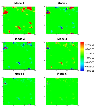
Figure 3.1: Two-dimensional field showing the first six dimensionless orthogonal

eigenfunctions for HO2 intermediate species mass fraction. ... 21

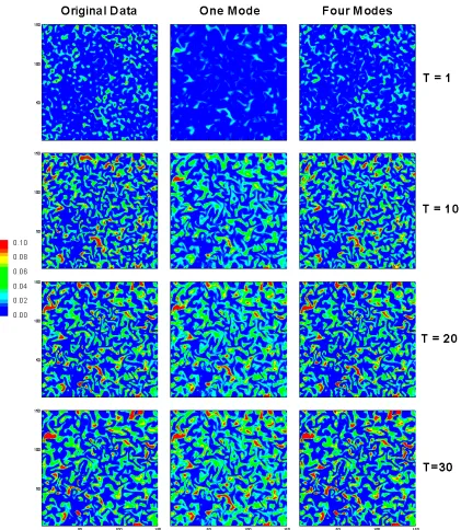
Figure 3.2: Two dimensional contour plot of mixture fraction showing the result of the POD reduction using one mode and four modes for times 1, 10, 20 and 30. ... 22 Figure 3.3: Two dimensional contour plot of progress variable showing the result of the

POD reduction using one mode and four modes for times 1, 10, 20 and 30. ... 23 Figure 3.4: Two dimensional contour plot of hydrogen reactant mass fraction showing the

result of the POD reduction using one mode and six modes for times 1, 10, 20 and 30... 24 Figure 3.5: Two dimensional contour plot of oxygen reactant mass fraction showing the

result of the POD reduction using one mode and six modes for times 1, 10, 20 and 30... 25 Figure 3.6: Two dimensional contour plot of H-radical mass fraction showing the result

of the POD reduction using one mode and six modes for times 1, 10, 20 and 30.... 26 Figure 3.7: Two dimensional contour plot of HO2 intermediate species mass fraction

showing the result of the POD reduction using one mode and six modes for times 1, 10, 20 and 30... 27 Figure 3.8: Magnitude of the Six Largest Eigenvalues and their Associated Energy

Percentage ... 28 Figure 3.9: Relative error of the POD unpreprocessed reduction for mixture fraction

showing the average error for each snapshot using various numbers of modes (1-6). ... 29 Figure 3.10: Relative error of the POD unpreprocessed reduction for progress variable

showing the average error for each snapshot using various numbers of modes (1-23, every third)... 30 Figure 3.11: Relative error of the POD unpreprocessed reduction for hydrogen reactant

showing the average error for each snapshot using various numbers of modes (1-6). ... 31 Figure 3.12: Relative error of the POD unpreprocessed reduction for oxygen reactant

showing the average error for each snapshot using various numbers of modes (1-9). ... 32 Figure 3.13: Relative error of the POD unpreprocessed reduction for H-radical showing

the average error for each snapshot using various numbers of modes (1-17 odd). .. 33 Figure 3.14: Relative error of the POD unpreprocessed reduction for HO2 intermediate

species showing the average error for each snapshot using various numbers of modes (1-23: every third)... 34 Figure 3.15: Correlation of POD reduced mixture fraction to original DNS results,

(9)

Figure 3.16: Correlation of POD reduced progress variable to original DNS results, showing an increase in the average correlation for each snapshot as the number of modes is increased ... 36 Figure 3.17: Correlation of POD reduced hydrogen reactant to original DNS results,

showing an increase in the average correlation for each snapshot as the number of modes is increased ... 37 Figure 3.18: Correlation of POD reduced oxygen reactant to original DNS results,

showing an increase in the average correlation for each snapshot as the number of modes is increased ... 38 Figure 3.19: Correlation of POD reduced H-radical to original DNS results, showing an

increase in the average correlation for each snapshot as the number of modes is increased ... 39 Figure 3.20: Correlation of POD reduced HO2 intermediate species to original DNS

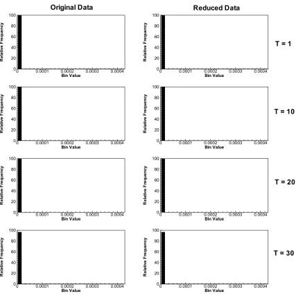
results, showing an increase in the average correlation for each snapshot as the number of modes is increased... 40 Figure 3.21: Histogram of original and unpreconditioned POD reduced mixture fraction

showing the relative frequency in percent for an even span of twenty locations for times 1, 10, 20 and 30. Notice only a slight variation in the resulting distribution after the POD reduction. ... 41 Figure 3.22: Histogram of original and unpreconditioned POD reduced progress variable

showing the relative frequency in percent for an even span of twenty locations for times 1, 10, 20 and 30. Notice a prominent variation in distribution; frequency and span. ... 42 Figure 3.23: Histogram of original and unpreconditioned POD reduced hydrogen

showing the relative frequency in percent for an even span of twenty locations for times 1, 10, 20 and 30. Notice only a slight variation in the resulting distribution after the POD reduction. ... 43 Figure 3.24: Histogram of original and unpreconditioned POD reduced oxygen showing

the relative frequency in percent for an even span of twenty locations for times 1, 10, 20 and 30... 44 Figure 3.25: Histogram of original and unpreconditioned POD reduced H-radical

showing the relative frequency in percent for an even span of twenty locations for times 1, 10, 20 and 30. Due to the low value of the majority of the data, the number of entries beyond the first value is minimal and des not show clearly. ... 45 Figure 3.26: Histogram of original and unpreconditioned POD reduced HO2 Intermediate

Species showing the relative frequency in percent for an even span of twenty

locations for times 1, 10, 20 and 30. ... 46

Figure 4.1: Relative error of the mean of the POD reduced mixture fraction for five different methods and up to six modes. ( ___ Unpreprocessed, ---- RMS

Preconditioned, -.-.-.- Mean Normalized, __ __ __ __ Max Normalized, -..-..-..- Log Preconditioned) ... 55 Figure 4.2: Relative error of the mean of the POD reduced progress variable for five

different methods and up to six modes. (Key is the same as Figure 4. 1) ... 56 Figure 4.3: Relative error of the mean of the POD reduced hydrogen for five different

(10)

Figure 4.4: Relative error of the mean of the POD reduced oxygen for five different methods and up to six modes. (Key is the same as Figure 4. 1) ... 58 Figure 4.5: Relative error of the mean of the POD reduced H-radical for five different

methods and up to six modes. (Key is the same as Figure 4. 1) ... 59 Figure 4.6: Relative error of the mean of the POD reduced HO2 intermediate species for

five different methods and up to six modes. (Key is the same as Figure 4. 1) ... 60 Figure 4.7: Relative error of the RMS of the POD reduced mixture fraction for five

different methods and up to six modes. (Key is the same as Figure 4. 1) ... 61 Figure 4.8: Relative error of the RMS of the POD reduced progress variable for five

different methods and up to six modes. (Key is the same as Figure 4. 1) ... 62 Figure 4.9: Relative error of the RMS of the POD reduced hydrogen for five different

methods and up to six modes. (Key is the same as Figure 4. 1) ... 63 Figure 4.10: Relative error of the RMS of the POD reduced oxygen for five different

methods and up to six modes. (Key is the same as Figure 4. 1) ... 64 Figure 4.11: Relative error of the RMS of the POD reduced H-radical for five different

methods and up to six modes. (Key is the same as Figure 4. 1) ... 65 Figure 4.12: Relative error of the RMS of the POD reduced HO2 intermediate species for

five different methods and up to six modes. (Key is the same as Figure 4. 1) ... 66 Figure 4.13: Correlation of mixture fraction as a result of the various preprocessing

techniques. The unpreprocessed result is shown for comparison. ( ___________ Unpreprocessed, --- Log Preconditioned, -.-.-.-.-.-.-.-.- Max Normalized, __

__ __ __ Mean Normalized, -..-..-..-..-..-..-..- RMS Preconditioned)... 67 Figure 4.14: Correlation of progress variable as a result of the various preprocessing

techniques. The unpreprocessed result is shown for comparison. (Key is the same as Figure 4.13) ... 68 Figure 4.15: Correlation of hydrogen as a result of the various preprocessing techniques.

The unpreprocessed result is shown for comparison. (Key is the same as Figure 4.13) ... 69 Figure 4.16: Correlation of oxygen as a result of the various preprocessing techniques.

The unpreprocessed result is shown for comparison. (Key is the same as Figure 4.13) ... 70 Figure 4.17: Correlation of H radical as a result of the various preprocessing techniques.

The unpreprocessed result is shown for comparison. (Key is the same as Figure 4.13) ... 71 Figure 4.18: Correlation HO2 intermediate species as a result of the various

preprocessing techniques. The unpreprocessed result is shown for comparison. (Key is the same as Figure 4.13)... 72 Figure 4.19: Histograms showing the variation of the relative frequency the three scalars,

mixture fraction, hydrogen and oxygen prior to POD reduction. The snapshot number is shown on the x-axis, the ‘bin value’ is shown in the y-axis and the

frequency (percentage) is indicated by the color contour... 73 Figure 4.20: Histograms showing the variation of the relative frequency of the progress

variable, H-radical and HO2 intermediate species scalars prior to POD reduction.

(11)

Figure A.1: Initial window for the POD GUI used in the data acquisition. ... 85

Figure A.2: After selecting the ‘Load’ option from the ‘DATA’ menu, the data size and the directory the data is located can be inputted an the various preconditioning and saving options can be chosen prior to selecting ‘PROCESS’... 86

Figure A.3: An example of a typical result... 86

Figure B.1: Preprocessed histogram comparison for mixture fraction. ... 87

Figure B.2: Preprocessed histogram comparison for hydrogen reactant species... 88

Figure B.3: Preprocessed histogram comparison for oxygen reactant. ... 89

Figure B.4: Preprocessed histogram comparison for H-radical... 90

(12)

Chapter 1

Introduction

1.1 Motivation

The prediction of non-linear transient phenomena in combustion presents important

challenges for the state-of-the-art models in turbulent combustion. Turbulent mixing and

combustion are governed by multiscale processes. At large scales, turbulent stirring

contributes to increasing entrainment and multiplying interfaces between scalars (e.g.

flames), while micro-mixing or molecular diffusion contributes to the dissipation of these

scalars. In combustion flows, the process of mixing is further coupled with the time

scales associated with combustion chemistry, giving rise to the so-called

‘turbulence-chemistry’ interactions. In statistically-transient combustion phenomena, such as

autoignition, the process is also governed by transitions in modes of combustion,

involving ignition to the formation of flames, which includes transitions in the dominant

chemistries associated with the induction and high-temperature combustion stages.

1.2 Direct Numerical Simulations Data and Proper Orthogonal Decomposition

The Direct Numerical Simulation (DNS) of reacting flows has long been useful to gain

fundamental insight into the physics of “turbulence-chemistry” interactions (Poinsot,

2000; Vervish and Poinsot, 1998). These interactions reflect the coupling between fluid

dynamics, chemistry, and molecular transport in multi-component mixtures. The theory

(13)

spatio-temporal DNS data of combustion phenomena. A reduced representation of this

data may provide a mechanism for the management and storage of DNS data for

post-processing and visualization. Moreover, it is possible to exploit these reduced

representations to develop low-order models of turbulence-chemistry interactions that

also reflect the transient character of important combustion processes such as ignition and

extinction. Tools that are based on dynamical systems theory have been proposed and

implemented in the field of fluid dynamics for more than thirty years (Lumley, 1967).

One such a tool is the Proper Orthogonal Decomposition (POD) technique. POD provides

a useful systematic characterization of patterns, such as coherent structures in shear

layers or ignition kernels in combustion, which are generated by non-linear phenomena

(Holmes, et al, 1997; Sirovich, 1987). These patterns may in turn be represented in lower

dimensional models, resulting in a significantly reduced description of these patterns. In

combustion, POD has been a useful tool to identify periodic and chaotic patterns in

burner-stabilized flames (Gorman, et al, 1994; Palacios et al, 1997; Palacios et al, 1996;

Palacios et al., 1998) and for data reduction of steady, 2D DNS data of opposed jet

flames by Frouzakis, et al (2000). These studies show that, depending on the nature of the

physics to be reproduced, the number of eigenmodes maintained can range from two to

five eigenmodes that account for the bulk of spectral energy. The wide range of

requirements for different combustion phenomena are strongly affected by two important

challenges in reproducing combustion data: transient effects and the multiscale nature of

(14)

1.3 Specific Content of DNS Data

The POD analysis is implemented on 2D DNS data of autoignition of a

non-homogeneous mixture of diluted hydrogen in heated air at 5 atmospheres, which were

carried out by Echekki & Chen (2003). The data consists of 2D spatial data on a

Cartesian grid and at equal time increments of thermo-chemical scalars. The fuel is a

50% H2/50% N2 mixture by volume at 300 K, and the oxidizer is air at 1180 K. The

mixture is maintained at a pressure of 5 atmospheres. The DNS data includes temporally

and spatially-resolved data for the thermodynamic state of the mixture including the

mixture composition consisting of 9 species, H2, O2, O, OH, H2O, H, HO2, H2O2, and N2,

whose chemistry is represented by a detailed mechanism of 19 elementary steps (Yetter,

et al, 1991). The resulting autoignition chemistry is consistent with the so-called second

explosion limit for hydrogen-air systems. The initial distribution of the mixture fraction

varies from pure fuel to pure oxidizer over a characteristic length scale, of 0.1 cm,

which is expressed in terms of the two-point correlation of the mixture fraction

fluctuations. A similarly-defined characteristic length scale for the velocity

fluctuations, , is set to 0.04 cm. The corresponding initial ‘turbulence’ intensity, u'', is

2.15 m/sec.

ξ L

u

L

The autoignition chemistry in the non-homogeneous mixture at the second explosion

limit is characterized by two stages: induction and high-temperature combustion. As

ignition kernels develop past the second stage, propagating fronts form to complete the

ignition process over the remaining unignited regions of the domain. The first stage of

(15)

absence of heat release (i.e. the absence of temperature rise due to combustion) (Kreutz

and Law, 1996). This stage is centered on the build-up of a radical pool through chemical

nonlinearity as opposed to thermal feedback. In the second stage, transition to

high-temperature combustion occurs, which is characterized by thermal runaway and the

establishment of a premixed flame front. Autoignition develops at discrete ignition sites

(or kernels) where the mixture state (temperature and composition) is most favorable to

the development of a radical pool and where the rates of dissipation of this radical pool

along with the dissipation of heat is lower than the rate of radical production. Because,

the initial stage of combustion is not associated with any significant heat release, tracking

the evolution of the radical pool is the primary indication of chemical activity during this

stage. HO2 is a reasonable marker of the level of chemical activity in the mixture and the

transition between the two stages of autoignition. Moreover, during these transitions, the

HO2 mass fraction displays significant changes over time. Similarly, the concentration of

radicals, such as H, O and OH, are direct measures of the evolution of the radical pool

during the induction stage. Therefore, reactive scalars are expected to evolve rapidly in

time during transitions between the two stages of autoignition and during the growth of

the autoignition kernels. In the present study, the initial configuration results in the first

onset of high-temperature combustion at 4x10-5 sec. By approximately 6x10-5 sec, most

of the igniting kernels have transitioned to the high-temperature combustion stage.

The computations are carried out to a stage where propagating ignition fronts form after

the onset of autoignition in discrete ignition kernels. The domain size is 0.37 cm by 0.37

cm, which is discretized with a Cartesian grid of 601 x 601 points. Therefore, the

(16)

consists of 30 snapshots of 2D fields of thermo-chemical scalars and velocity vector

components provided at equal time increments of 2.15 x 10-6 sec, and ranging from 2.15

x 10-6 to 6.67 x 10-5 sec. The final time corresponds to the completion of the induction

process in the bulk of ignition kernels, and the onset of high-temperature combustion.

1.4. Objectives

While there is reasonable understanding of the relevance and limitations of the POD

approach to turbulent nonreacting flows, an understanding of the value of POD in

turbulent combustion remains limited. The bulk of POD reduction has been carried out on

relatively coarse (in space) experimental observables including, for example, velocity

data from Particle Image Velocimetry, visible flame emissions or fluorescence signals.

Highly utilized in stead-state problems, POD has not been fully analyzed in unsteady

fine-grain numerical data. Moreover, different POD reduction requirements are reported

to address different scalars and velocity components. Invariably, there should be different

POD reduction requirements for the prediction of different phenomena, especially during

highly transient processes, and the reproduction of different quantities. The relative

complexity necessary to capture transient, multi-component and multiscale processes

requires the development of different processing strategies to reduce the required number

of POD modes.

The objectives of this study are a) to evaluate requirements for the reproduction of DNS

data of the autoignition of hydrogen with heated air in a non-homogeneous mixture and

b) to explore whether different preprocessing strategies for the scalar fields can reduce

(17)

of many simulations involving strongly transient phenomena with wide scale variations.

Reduced representations of DNS data may be exploited to store and manage these data

sets for post-processing and visualization. They may also be used to develop low-order

models that accurately represent transient phenomena in combustion. These models may

then be coupled with a coarse-grained simulation, such as Reynolds Averaged

Navier-Stokes (RANS) or Large Eddy Simulation (LES) approaches.

1.5. Thesis Outline

The DNS data and the POD approach are detailed in Sections 1.3 and 1.4 respectfully.

The following section includes a description of proper orthogonal decomposition and its

multitude of uses. Next, results of the POD analysis for the passive scalar, mixture

fraction and reactive scalars; the reaction progress variable, hydrogen, oxygen, H-radical

and HO2 species mass fractions are presented and discussed first to illustrate the process

of POD reduction for the autoignition data (Section 2.1). This is followed by a discussion

of the effects of different preprocessing strategies for the reduction of passive and

reactive scalars data (Section 2.2). The results of the un-preprocessed reduction of the

auto-ignition data is shown in chapter three, while the preprocessed results are shown in

chapter four. Finally, conclusions are presented on the validity of the POD approach and

(18)

Chapter 2

The POD Reduction Approach

2.1. POD

Customarily, spatio-temporal data is represented by a large system of ordinary

differential equations (ODE’s). The solution to this large system of equations would

customarily require the direct solution to each of these ODE’s however; this system may

be represented by a reduced set of ODE’s using a Galerkin procedure (Frouzakis, et al

2000). This highly efficient and adaptable reduction technique has been used in many

different fields, including signal processing, pattern recognition, structural vibrations,

damage detection and fluid flow (Cusumano, et al, 1994; Sirovich, 1987; Ruotolo and

Surace 1999). Much like in signal processing (Hua and Liu, 1998), POD can be used to

compress and filter computational combustion data and has been effective in developing

coherent structures in dynamic particle image velocimetry (DPIV), where data size is

comparable to that of DNS (Kodal, et al, 2003 ; Bi et al, 2003). POD has also been

shown to be more effective than standard Fourier methods in when representing highly

chaotic flows (Rajaee, et al., 1993). The process of POD reduction has a variety of

different variations which include the derivation from spatial correlations or conditional

measurements (Delville, 1993). Presented here is the method of snapshots originally

developed by Sirovich (1987).

Using a MATLAB written graphical user interface (GUI), the POD method is applied on

DNS data, which represents a 2D spatial resolution of discrete grid-resolved velocity and

(19)

(See Appendix A for a description of the use of the MATLAB code). The DNS data is

organized as a matrix containing spatio-temporal data, where the spatial variation can be

seen as a column vector of size, N. The temporal variation is represented in the different

rows of the matrix with M rows, corresponding to the different temporal snapshots:

. ..., , 1 ...,

,

1 N j M

i

X_ij = = (2.1)

In this equation, X corresponds to the matrix values of the desired scalar field; the index,

i, corresponds to the spatial coordinate along the column vector of discrete x and y

locations for the grid points; and the subscript j corresponds to the discrete time of the

snapshot. The character vectors are computed using a specific preprocessing technique

discussed in subsection 2.2:

data DNS processed

X_i.≡ . (2.2)

i ij ij

X X

Xˆ = _(2.3)

Using the method of snapshots developed by Sirovich (1987), where the temporal

‘snapshot’ contains a basis which reflects the dynamics of the system, the covariance

matrix is evaluated using:

. ..., , 1 ...,

, 1 ˆ

ˆ _X _i _M _j _M

X

C_ij = _i• _j = = (2.4)

The eigenvalues and eigenvectors can then be evaluated from the covariance matrix. The

eigenfunctions may be expressed as:

, ,..., 1

ˆ _j _M

X

j

j =φ =

ψ (2.5)

where φ_j is the jth eigenvector and _ψ( )j _{is the}_jth_{row eigenfunction. The eigenfunctions}

(20)

reconstruct the data (Armbruster, et al, 1993). Assuming the eigenvalues represent the

spectral energy of the system and that they are organized from most energetic to least

(largest to smallest), then the sum of all the eigenvalues would give the total energy of

the system:

∑

=

= M

i i

E

1

λ , (2.6)

where λ_i is the ith_{eigenvalue. An associated energy percentage for each eigenvalue can}

be found:

E

E i

i

λ

= , where λ₁ >λ₂ >...>λ_M >0. (2.7)

The temporal coefficients needed to represent the temporal flux of the data can be defined

as:

( )

_.

ˆ

k k

T k T i i

X a

ψ ψ

ψ • •

= (2.8)

Using these newly evaluated coefficients, the estimated data can be found using the most

R energetic eigenfunctions (R < M):

. 1

∑

=

+

= R

k k k i

ij X a

X ψ (2.9)

The POD reduced data can then be compared to the original data by calculating a percent

difference for each time step and mapping the relative error to the appropriate location on

the grid. This method of error calculation, however, fails to capture accurately the

representation when the original field magnitude approaches zero. Therefore other error

(21)

can also be determined in order to ascertain the difference between the original and

constructed data.

In order to reduce a two dimensional unsteady field with multiple temporal values using

POD, the data needs to be reorganized. This is done by concatenating the rows of the

spatial field so the sequential row at the same column is still neighboring the value that

was previously above it and then placing these vectors, column-wise into a matrix. This

results in what is called contiguous concatenation (Figure 2.1). This method allows for a

more accurate approximation due to the continuous variation that occurs along the

resulting vector. Once completed for each time step, the resulting matrix will be

(assuming a square spatial matrix)M2 X N.

2.2 Preprocessing Techniques

The representation of temporal and spatial variations of scalar data during the

autoignition process using POD may require the use of a large number of eigenvalues and

associated eigenmodes because of the multiscale nature of these variations. In this work,

four different strategies are implemented to reduce the number of required eigenvalues to

represent the data through preprocessing of the scalar field.

• Method I: The first method is based on a simple implementation of the logarithmic

function on the scalar field. The POD procedure, Eqs. (2.2)-(2.9), is therefore

implemented on the natural logarithmic values of the scalar field matrix elements, Xij:

) log( ˆ

ij

ij X

(22)

Method II: The second method consists of normalizing the scalar field values by the

maximum values (X~_ij) at a given snapshot.

, ~ ˆ

ij ij ij

X X

X = where _j max _ij for all

j

X% = X i (2.11)

Method III: The third method is based on the normalization of the scalar field by the

mean computed for the same snapshot (of time) to yield unity mean character vector:

ˆ ij_, ij

j

X X

X

= where

1 1

,

N

j i

ij

X X

N =

=

∑

(2.12)

where X_j is the mean value of the scalar field at a given snapshot (time). Therefore, the

preprocessing associated with this method consists of simply shifting the mean of the

scalars to zero. Method III is expected to yield comparable values of the means of the

character vectors. However, it does not address the deviation of the scalar field values

around this mean. More importantly, the method is expected to yield comparable values

for the different snapshots only if the means are close to the peak distributions of the

values of the scalar data. Therefore, a bimodal or more complex probability density

function (PDF) distribution associated with a highly transient process such as ignition or

extinction for reactive scalars may not provide significant improvements for the

pre-processing method III.

• Method IV: The fourth method is based on reducing the initial scalar field to the

following form prior to POD reduction:

ˆ ij j _,

ij

j

X X

X

− =

′′ where

( )

2 2

1

, N

j ij

i

X X X

N =

(23)

where X′′_j is the RMS value of the scalar field at a given snapshot (time). Therefore, in

contrast to the third method (or method III), the above transformation modifies both the

location of the mean and the distribution of the modified scalar field. In accordance with

the above argument related to method III, method IV is expected to provide comparable

distributions for the scalar fields only when these distributions are simple, such as

Gaussian or log-normal.

Except for method I, the remaining methods require prior knowledge of at least one

moment or a peak value of the scalar statistics to reproduce the original field. These

moments are computed using the DNS data, and in practice are assumed to be evaluated

using transport equations for the first moments of the scalar. The transport equations are

normally evaluated using coarse-grained approaches to turbulent combustion (eg. LES or

RANS) for, at least, the mixture fraction.

2.3 Assessment of the Performance of the Different Preprocessing Approaches

The most common criterion for the evaluation of the total number of modes required to

reproduce original computational or experimental data is based on the cumulative energy

percentage expressed in Eq. (2.7) (Holmes, et al, 1997). However, this energy criterion is

consistent with the dominant patterns of the data, in contrast with the range of values

typical autoignition data represents. Therefore, this criterion may not be sufficient to

characterize the reduction process associated with the capturing of the ‘entire’ range of

scalar data of interest here. However, to reproduce autoignition data, an accurate

representation of a wide range of spatial and temporal scales is needed. The general

(24)

data can be used as an indication of successful representation. This is done with the

correlation. The correlation, Cj, is expressed as follows:

(

)

(

)

(

)

∑

⋅ ⋅

⋅

⋅ =

i i

POD ij POD ij orig

ij orig ij

i

POD ij orig ij

j

X X X

X

X X

C (2.14)

While able to define the ‘quantity’ (general similarity) between the two data sets, this

method does not however, completely describe the quality of the accuracy. Therefore a

percent error method is used in the following chapter to directly determine the variations

at each location on the plane:

DNS j

DNS j POD j j

X X X

E = − , (2.15)

where the superscript POD is the result from the POD reduction and DNS is the original

DNS data. Due to the low magnitudes of the original DNS values however, a direct

percent error or relative error results in erroneous inaccuracy; exaggerating the variations

in the low-scale regions. The following measures have therefore been adopted to

evaluate the quality of the POD reduction approach for unprocessed and preprocessed

passive and reactive scalars’ data and are presented in chapter four. These are:

• The relative error associated with the spatial means of the scalar at a given snapshot

of time:

DNS j

DNS j POD j mean j

X X X

E = − (2.16)

where the superscripts, POD and DNS, refer to the POD reduced data and the DNS data,

(25)

• The relative error associated with the spatial fluctuations (rms) of the scalar at a given

snapshot of time:

DNS j

DNS j POD j mean j

X X X

E

′′ ′′ − ′′

= (2.17)

The two parameters, mean and

j

E rms

j

E , provide global measures of the error associated with

the reproduction of the mean and the spread of the data as a function of time.

(26)

Chapter 3

Results: Investigation of POD Reduction

Requirements for Spatio-Temporal Data

in Combustion

The following section presents results pertaining to the proper orthogonal decomposition

of the spatio-temporal data recovered from a direct numerical simulation of the

autoignition of hydrogen and air. Due to their varying statistics and areas of

concentrations, six different spatio-temporal fields are investigated to determine the

requirements of the POD reproduction. The data includes: the mixture fraction (Z), the

reaction progress variable (C), and the mass fraction of H2, O2, H and HO2.

While there are multiple definitions of the mixture fraction, Z, the Bilger mixture fraction

definition has been used (Bilger et al, 2003):

, ,

, , , ,

( ) / 2 ( ) /

,

( ) / 2 ( ) /

H H o H O O o O

H f H o H O f O o O

Y Y W Y Y W

Z

Y Y W Y Y W

− − −

=

− − − (3.1)

where Y’s are the elemental mass fractions, W’s are atomic weights and the subscripts, f

and o, correspond to the fuel mixture and air, respectively.

Characterized as a nonconserved tracking scalar, the reaction progress variable measure

the extent of completion of reaction, and is normalized as such it is equal to zero on the

reactants’ side and unity on the products side. Intermediate values of the reaction

progress variable can be used to determine the location of flame fronts, and therefore

(27)

many forms, but is defined here as a normalization of the various temperatures associated

with the reactants. The following equation is the definition of progress variable used in

this study:

unburned adiabatic

unburned

T T

T T C

− −

= , (3.2)

where is adiabatic flame temperature corresponding to the burning of a fuel and

oxidizer mixture to chemical equilibrium at a prescribed mixture fraction, which

corresponds to the local computed Bilger mixture fraction value at the same location. The

mixture composition and temperature, T , of the reactants’ mixture is obtained

assuming an adiabatic mixing process at constant pressure. Because the mixture fraction

uniquely determines the reference unburnt,T final equilibrium temperatureT

can be tabulated as a function of mixture fraction.

adiabatic

T

unburned

unburned adiabatic

3.1 Requirements of Reconstruction of Spatio-Temporal Data of Autoignition for

Passive and Reactive Scalars

In order to observe the direct variation between the original and POD reduced data, a

visual comparison must be performed. Figure 3.2 through Figure 3.7 contrast the original

and reduced 2D unprocessed fields of the mixture fraction (Z), the reaction progress

variable (C), and the mass fractions of H2, O2, H and HO2 at four different times

corresponding to the induction and the high-temperature stages of autoignition. The

figures show that the POD reduced fields reproduce reasonably of the overall topology of

(28)

With only a visual inspection, the mixture fraction can be well reproduced with four

modes as shown in Figure 3.2. When observing the visual field of the reproduction of H2

and O2, the necessity to increase the number of modes becomes clear (Figure 3.4 and

Figure 3.5) Unlike the mixture fraction field, reactant species, H2 and O2, show a more

accurate representation during the initial times due to their higher concentration during

these times. The initial non-homogeneous field is made up of different ‘islands’ of peak

concentrations of H2, surrounded by regions of low concentrations of H2 (as shown in

Figure 3.4). A similar topology is also seen for the oxidizer, O2.

For species with low concentrations during the induction stage, H and HO2, the reduced

data is significantly different from the original data during these early stages of the

autoignition process (the first snapshot in the figure) and at limited regions for the other

snapshots. As shown in the figures (Figure 3.6 and Figure 3.7), the most significant

departure from the original data corresponds to regions of relatively low concentrations

and outside or at the periphery of the autoignition kernels.

This can be compared to DNS data from a steady state opposed-jet diffusion flame

(Frouzakis; et al, 2000). The results of this study concluded only six to nine modes are

required to represent HO2 intermediate species mass fraction to within 25% relative error.

However, the transient nature of the present autoignition data may impose more stringent

requirements on the number of modes needed to reproduce the early stages of

autoignition. These requirements are the primary motivation for exploring different

preprocessing strategies for the DNS data. Moreover, it is important to explore other

(29)

3.2 Analysis of Performance of the POD Reduction Approach for passive and reactive scalars using relative error and correlation

In order to show the contribution of each mode, a bar chart of these contributions is used.

Figure 3.8 shows the magnitudes of the six largest eigenvalues associated with the POD

reduction of the unprocessed HO2 mass fraction fields. HO2 was chosen due to its

important role as a common indicator of reaction during the two stages of autoignition.

Also shown in the figure are the cumulative energy percentages of the eigenvalues (Eq.

2.7). While the spectral energy alone does not describe the accuracy of the reduction, it

does give some insight into the amount of reduction occurring. The figure shows the

large contribution of the largest eigenvalues; where the first three alone account for 90%

of the spectral energy; while, the remaining eigenvalues make up only 10% of the

spectral energy. With three additional eigenvalues, which represent a total of the six

largest eigenvalues, 98.5% of the spectral energy is reproduced. The remaining low

dimensional modes remained unused. Since the exact accuracy of the reduction

technique is not completely defined by the spectral energy, another method must be used

to determine if the POD reduced data is accurate compaired to the original. This was

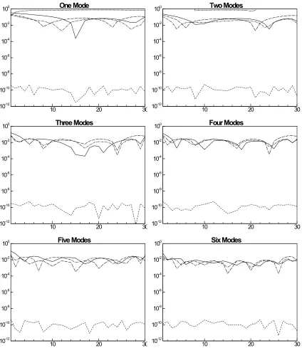
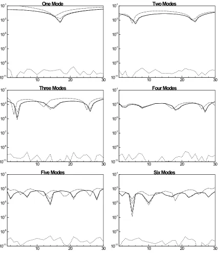
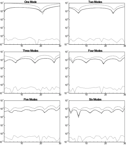
done using the relative error.

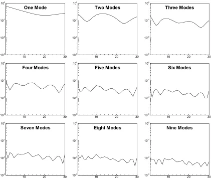
The relative error is an appropriate method for determination of accuracy between two

similar scalar fields. The average relative error is shown in Figure 3.9 through Figure

3.14 along the temporal direction. According to Figure 3.9 and Figure 3.10, moderately

varying species like mixture fraction and progress variable, require only four to five

(30)

The remaining highly varying species however, require more modes to represent than

species which posses low fluctuations. According to Figure 3.11 through Figure 3.14,

hydrogen requires six modes, oxygen requires eight to nine modes, H-radical requires

sixteen to seventeen modes and HO2 requires the most at twenty-two to twenty-three

modes. This method of error determination however, can be inaccurate. When the

magnitude of the scalars is minimal, the division by the unreduced DNS data can produce

inaccurate, high valued error (Eq. 2.16). Other approaches must be utilized in order to

compensate for this inaccuracy.

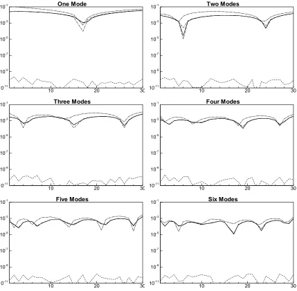
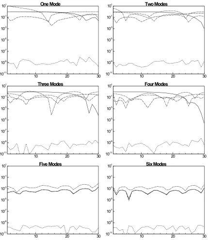
The correlation is a useful method to determine the similarity in trends between the two

data sets (Figure 3.15 through Figure 3.20). According to Figure 3.15, the number of

modes required to correlate the POD reduced mixture fraction with the original a near

singular value is only three. This agrees with the previous figure (Figure 3.9) of the

mixture fraction. This agreement is short lived as Figure 3.16 shows the requirements to

correlate progress variable. As shown, the progress variable requires many more modes

to be reproduced than previously shown. With the exception of hydrogen (Figure 3.17),

the remaining species show a similar trend, where the correlation shows the necessity to

increase the number of modes to accurately describe the temporal variations of the data.

The resulting method therefore, becomes an “interpolation” between these two

techniques. Initially monitoring the average relative error and cross-referencing that

value with the correlation can give the observer a closer approximation to the accuracy of

the POD technique. Unfortunately this is not enough to accurately determine if the POD

(31)

be explored to determine accuracy, including an investigation into the statistical

variations occurring in the data.

3.3. The Importance of the Statistical Distribution to the POD Reconstruction Accuracy

Often used to show a visual display of the relative frequency of observations which fall

into a particular class (Moore and McCabe, 2001), the relative frequency histogram

shows the general shape of the percent of observations This shape is essential to the

accuracy of the reduction, when compared for each time. The distribution of the mixture

fraction (Figure 3.21) and hydrogen reactant (Figure 3.23) can be described as skewed to

the right or positively skewed, meaning there is a separation of the mean and the median.

Figure 3.24 shows the histogram of the distribution of oxygen reactant. This distribution

can be described as negatively skewed, meaning the median is less than the average. A

species showing a skew near zero is said to be more “normal” and as a result, a more

accurate POD representation is possible. The distribution of the H-radical (Figure 3.25)

and HO2 (Figure 3.26) intermediate species is highly positively skewed. Since this skew

is coupled with a very low magnitude mean, the accuracy of the POD representation must

be determined by other methods. Since there is a definite separation of acceptable POD

representation accuracy and correlation to the original trends, as well as a questionable

statistical distribution, especially with species that show highly skewed data sets,

techniques must be developed to allow a more accurate POD representation while

maintaining a low number of modes. The next chapter presents the results from a variety

(32)

(33)

(34)

(35)

(36)

(37)

(38)

(39)

(40)

10 20 30 0.1

0.2 0.3 0.4 0.5

0.6

_{One Mode}

10 20 30

0.02 0.04 0.06 0.080.1 0.12 0.14

Three Modes

10 20 30

0.02 0.04 0.06 0.080.1 0.12 0.14

Five Modes

102030 10 20 30

0.02 0.04 0.06 0.080.1 0.12

0.14

Two Modes

10 20 30

0.02 0.04 0.06 0.080.1 0.12 0.14

Four Modes

10 20 30

0.02 0.04 0.06 0.080.1 0.12 0.14

Six Modes

(41)

10 20 30 104

105

106

107

10

Seven Modes

10 20 30 104

105

106

107

108

Ten Modes

10 20 30 104

105

106

107

108

13 Modes

10 20 30 104

105

106

107

108

16 Modes

10 20 30 104

105

106

107

108

19 Modes

10 20 30 104

105

106

107

108

22 Modes

10 20 30 104

105

106

107

108

23 Modes 10 20 30

104

105

106

107

10

Four Modes

10 20 30 104

105

106

107

10

One Mode

(42)

10 20 30 10-3

10-2

10-1

100

Three Modes

10 20 30

10-3

10-2

10-1

100

Four Modes

10 20 30

10-3

10-2

10-1

100

Five Modes

10 20 30

10-3

10-2

10-1

100

Six Modes

10 20 30

10-3

10-2

10-1

100

One Mode

10 20 30

10-3

10-2

10-1

100

Two Modes

(43)

10 20 30 10-3

10-2

10-1

10

One Mode

10 20 30 10-3

10-2

10-1

10

Two Modes

10 20 30 10-3

10-2

10-1

10

Three Modes

10 20 30 10-3

10-2

10-1

100

Four Modes

10 20 30 10-3

10-2

10-1

100

Five Modes

10 20 30 10-3

10-2

10-1

100

Six Modes

10 20 30 10-3

10-2

10-1

100

Seven Modes

10 20 30 10-3

10-2

10-1

100

Eight Modes

10 20 30 10-3

10-2

10-1

100

Nine Modes

(44)

10 20 30 10-3

10-2

10-1

10

1 Mode

10 20 30 10-3

10-2

10-1

10

3 Modes

10 20 30 10-3

10-2

10-1

10

5 Modes

10 20 30 10-3

10-2

10-1

100

7 Modes

10 20 30 10-3

10-2

10-1

100

9 Modes

10 20 30 10-3

10-2

10-1

100

11 Modes

10 20 30 10-3

10-2

10-1

100

13 Modes

10 20 30 10-3

10-2

10-1

100

15 Modes

10 20 30 10-3

10-2

10-1

100

17 Modes

(45)

10 20 30 10-3

10-2

10-1

10

1 Mode

10 20 30 10-3

10-2

10-1

10

4 Modes

10 20 30 10-3

10-2

10-1

10

7 Modes

10 20 30 10-3

10-2

10-1

100

10 Modes

10 20 30 10-3

10-2

10-1

100

13 Modes

10 20 30 10-3

10-2

10-1

100

16 Modes

10 20 30 10-3

10-2

10-1

100

19 Modes

10 20 30 10-3

10-2

10-1

100

22 Modes

10 20 30 10-3

10-2

10-1

100

23 Modes

(46)

Snapshot

10 20 30

0.6 0.65 0.7 0.75 0.8 0.85 0.9 0.95 1

Snapshot

10 20 30

0.6 0.65 0.7 0.75 0.8 0.85 0.9 0.95 1

Snapshot

10 20 30

0.6 0.65 0.7 0.75 0.8 0.85 0.9 0.95 1

Snapshot

10 20 30

0.6 0.65 0.7 0.75 0.8 0.85 0.9 0.95 1

One

Mode

Modes

Four

Modes

Two

Modes

Three

(47)

Snapshot

10 20 30

0.2 0.4 0.6 0.8 1

Snapshot

10 20 30

0.2 0.4 0.6 0.8 1

Snapshot

10 20 30

0.2 0.4 0.6 0.8 1

Snapshot

10 20 30

0.2 0.4 0.6 0.8 1

One

Mode

Modes

Four

Modes

Two

Modes

Three

(48)

Snapshot

10 20 30

0.7 0.75 0.8 0.85 0.9 0.95 1

Snapshot

10 20 30

0.7 0.75 0.8 0.85 0.9 0.95 1

Snapshot

10 20 30

0.7 0.75 0.8 0.85 0.9 0.95 1

Snapshot

10 20 30

0.7 0.75 0.8 0.85 0.9 0.95 1

One

Mode

Modes

Four

Modes

Two

Modes

Three

(49)

Snapshot

10 20 30

0.7 0.75 0.8 0.85 0.9 0.95 1

Snapshot

10 20 30

0.7 0.75 0.8 0.85 0.9 0.95 1

Snapshot

10 20 30

0.7 0.75 0.8 0.85 0.9 0.95 1

Snapshot

10 20 30

0.7 0.75 0.8 0.85 0.9 0.95 1

One

Mode

Modes

Four

Modes

Two

Modes

Three

(50)

Snapshot

10 20 30

0.6 0.65 0.7 0.75 0.8 0.85 0.9 0.95 1

Snapshot

10 20 30

0.6 0.65 0.7 0.75 0.8 0.85 0.9 0.95 1

Snapshot

10 20 30

0.6 0.65 0.7 0.75 0.8 0.85 0.9 0.95 1

Snapshot

10 20 30

0.6 0.65 0.7 0.75 0.8 0.85 0.9 0.95 1

One

Mode

Modes

Four

Modes

Two

Modes

Three

(51)

Snapshot

10 20 30

0.6 0.65 0.7 0.75 0.8 0.85 0.9 0.95 1

Snapshot

10 20 30

0.6 0.65 0.7 0.75 0.8 0.85 0.9 0.95 1

Snapshot

10 20 30

0.6 0.65 0.7 0.75 0.8 0.85 0.9 0.95 1

Snapshot

10 20 30

0.6 0.65 0.7 0.75 0.8 0.85 0.9 0.95 1

One

Mode

Modes

Four

Modes

Two

Modes

Three

(52)

Bin Value R e la ti ve F re q ue nc y

0 0.2 0.4 0.6 0.8 1

0 2 4 6 8 10 Bin Value R e la tiv e F re q ue nc y

0 0.2 0.4 0.6 0.8 1

0 2 4 6 8 10 Bin Value R e la ti ve F re q ue nc y

0 0.2 0.4 0.6 0.8 1

0 0.25 0.5 0.75 1

0 0.2 0.4 0.6 0.8 1

0 2 4 6 8 10

T = 1

T = 10

T = 20

T = 30 Reduced Data

Original Data

(53)

Bin Value R e la tive F re que n cy

0 0.2 0.4 0.6 0.8 1 0 20 40 60 80 100 Bin Value Re la tiv e F re q u e n cy

0 0.25 0.5 0.75 1 0 20 40 60 80 100 Bin Value Re la tiv e F re q u e n cy

0 0.25 0.5 0.75 1 0 20 40 60 80 100 Bin Value R e la tive F re que n cy

0 0.1 0.2 0.3

0 20 40 60 80 100 Bin Value Re la tiv e F re q u e n cy

0 0.1 0.2 0.3

0 20 40 60 80 100

T = 1

T = 10

T = 20

T = 30 Reduced Data

Original Data

(54)

0 0.01 0.02 0.03 0.04 0.05 0.06 0.07 0 2 4 6 8 10 Bin Value Re la tiv e F re q u e n cy

0 0.01 0.02 0.03 0.04 0.05 0.06 0.07 0 2 4 6 8 10 Bin Value R e la tive F re que n cy

0 0.01 0.02 0.03 0.04 0.05 0.06 0.07 0 2 4 6 8 10

Original Data Reduced Data

T = 1

T = 10

T = 20

T = 30

(55)

0 0.05 0.1 0.15 0.2 0 2 4 6 8 10 Bin Value Re la tiv e F re q u e n cy

0 0.05 0.1 0.15 0.2 0 2 4 6 8 10 Original Data Bin Value R e la tive F re que n cy

0 0.05 0.1 0.15 0.2 0 2 4 6 8 10 Reduced Data

T = 1

T = 10

T = 20

T = 30

(56)

0 0.0001 0.0002 0.0003 0.0004 0 20 40 60 80 100 Original Data Bin Value Re la tiv e F re q u e n cy

0 0.0001 0.0002 0.0003 0.0004 0 20 40 60 80 100 Bin Value R e la tive F re que n cy

0 0.0001 0.0002 0.0003 0.0004 0 20 40 60 80 100 Reduced Data

T = 1

T = 10

T = 20

T = 30

(57)

0 0.0001 0.0002 0.0003 0.0004 0 20 40 60 80 100 Bin Value R e la tive F re que n cy

0 0.0001 0.0002 0.0003 0.0004 0 20 40 60 80 100

Original Data Reduced Data

T = 1

T = 10

T = 20

T = 30

(58)

Chapter 4

Effect of Preprocessing of DNS Data on

POD Reduction Requirements

In the previous chapter, the ‘raw’ POD reduction procedure resulted in relatively

stringent requirements on the number of mode required to represent the data. Moreover,

the different measures of error show fundamentally different POD reduction requirements

for the different scalars (reactive and passive). In this chapter, we explore the effects of

preprocessing of the data on POD reduction in the aim of reducing the requirements on

the number of modes.

The following section introduces the results of the preprocessing modifications applied to

the spatial-temporal DNS data. Each species is sorted and modified according to the

techniques described in section 2.2. After preprocessing, the POD reduction technique is

applied. Due to the low magnitude associated with a majority of the data, standard

relative error analysis is not presented graphically. Accuracy is determined by proximity

to mean and rms as previously described above. The statistical distribution of the data is

analyzed to suggest a correlation between normality and POD reduction accuracy. A

table summarizing the effectiveness of each of the preconditioning techniques is shown at

the end of the chapter for ease of comparison (see Table 4.2). An ‘accurate’

representation is considered to be a representation resulting in less than 5% variation for

(59)

4.1 Required Preconditioning to Reduce the Low-Order POD Model

Figure 4.1 through Figure 4.6 show the temporal evolution of the global relative error of

the mean of the scalar fields based on Eq. (2.14) for a range of combined modes from 1

through 6 and for the different preprocessing strategies discussed in the section 2.2. The

success of the preprocessing techniques depends upon the species explored. According

to Figure 4.1 the POD reduction of the mixture fraction most successfully approximates

the mean when preconditioned by method IV (RMS), which is based on the

normalization of the data, shifted with respect to its mean, by the RMS value. This value

does not display in the figure due to the extremely low valued error ( ); in this

range round-off error overwhelms the value of the relative error. For this method, a

single mode is sufficient to reproduce the mean of the data well. Aside from the log

preconditioning, the remaining methods perform similarly with accuracy varying little

from the unpreconditioned values.

(

−11

Θ

)

Figure 4.2 shows the preprocessed POD reduction for progress variable. In this instance,

two techniques are not clearly shown due to their high variation. These include method I

(log preconditioning) which has extremely high error (Θ

( )

1 toΘ

( )

4 ) and method IV

which has extremely low error

(

Θ

(

−10

)

. Compared to the other methods, method IV is

more accurate and can approximate the original field using only one mode. The

remaining figures show very similar results to those of the mixture fraction and progress

variable. Method IV is the most accurate preprocessing technique to allow a more

accurate POD reconstruction of the mean with fewer modes for all the species except

(60)

species is best approximated after the POD reduction using method II (maximum

normalization), which can accomplish this high accuracy with only six modes.

Figure 4.7 through Figure 4.12 show the temporal evolution of the global relative error of

the scalar fields based on Eq. (2.17). In order to represent the range of mixture fraction

data, Figure 4.7 suggests preconditioning is unnecessary when four modes are used.

There appears to be no significant advantage to the other preprocessing strategies;

although, method I, based on the POD reduction of the logarithmic function of the

mixture fraction, yields the highest error. POD reduction that is based on unprocessed

and modified mixture fraction fields using methods II and III requires approximately

three to four modes to yield accurate relative errors for both mean and rms. Therefore,

the overall most accurate preprocessing technique for the mixture fraction is method IV,

with a POD reconstruction utilizing only four modes. The accuracy of the range of the

progress variable data that the various preprocessing techniques influence the POD

reduction is shown in Figure 4.8. The figure shows the necessity to use six modes

regardless of the technique used. However, log-preconditioning fails to accurately

represent the original DNS progress variable with any reasonable number of eigenmodes.

The range of the progress variable is best reproduced when preconditioned using method

IV according to the figure, resulting in that method being the overall most accurate

preconditioning strategy when six modes are used. The remaining reactive scalars

require the same preconditioning method be applied to increase accuracy, which is

method II. For many of these scalars, there is little variation between the different

approaches, resulting in the overall most effective preconditioning technique being

Optimization of Proper Orthogonal Decomposition using Various Preconditioning Techniques to Analyze Autoignition Simulation Data of Non-Homogeneous Hydrogen-Air Mixtures

Non-Homogeneous Hydrogen-Air Mixtures

Mechanical Engineering

Biography

Acknowledgment

Contents

List of Tables

List of Figures

Chapter 1

Introduction

Chapter 2

The POD Reduction Approach

∑

( )

∑

∑

( )

(

)

(

)

(

)

∑

∑

∑

Chapter 3

Results: Investigation of POD Reduction

Requirements for Spatio-Temporal Data

in Combustion

One Mode

Three Modes

Five Modes

Two Modes

Four Modes

Six Modes

Three Modes

Four Modes

Five Modes

Six Modes

One Mode

Two Modes

One

Mode

Modes

Four

Modes

Two

Modes

Three

One

Mode

Modes

Four

Modes

Two

Modes

Three

One

Mode

Modes

Four

Modes

Two

Modes

Three

One

Mode

Modes

Four

Modes

Two

Modes

Three

One

Mode

Modes

Four

Modes

Two

_{One Mode}