ABSTRACT
BEELER, SCOTT COLVIN. Modeling and Control of Thin Film Growth in a Chemical Vapor
Deposition Reactor. (Under the direction of Hien T. Tran.)
This work describes the development of a mathematical model of a high-pressure chemical vapor
deposition (HPCVD) reactor and nonlinear feedback methodologies for control of the growth of thin
films in this reactor. Precise control of the film thickness and composition is highly desirable, making
real-time control of the deposition process very important. The source vapor species transport is
modeled by the standard gas dynamics partial differential equations, with species decomposition
reactions, reduced down to a small number of ordinary differential equations through use of the
proper orthogonal decomposition technique. This system is coupled with a reduced order model
of the reactions on the surface involved in the source vapor decomposition and film deposition on
the substrate wafer. Also modeled is the real-time observation technique used to obtain a partial
measurement of the deposition process.
The utilization of reduced order models greatly simplifies the mathematical formulation of the
physical process so it can be solved quickly enough to be used for real-time model-based feedback
control. This control problem is fairly complicated, however, because the surface reactions render
the model nonlinear. Several control methodologies for nonlinear systems are studied in this work
to determine which performs best on test examples similar to the HPCVD problem. One chosen
method is extended to a tracking control to force certain film growth properties to follow desired
trajectories. The nonlinear control method is used also in the development of a state estimator
which uses the nonlinear partial observation of the nonlinear system to create an estimate of the
actual state, which the feedback control formula then can use to guide the HPCVD system. The
nonlinear tracking control and estimator techniques are implemented on the HPCVD model and the
MODELING AND CONTROL OF THIN FILM GROWTH
IN A CHEMICAL VAPOR DEPOSITION REACTOR
by
Scott Colvin Beeler
a dissertation submitted to the graduate faculty of
north carolina state university
in partial fulfillment of the
requirements for the degree of
doctor of philosophy
applied mathematics
raleigh
October 2000
approved by:
H. T. Tran H. T. Banks
chair of advisory committee
Biography
Scott Colvin Beeler was born and raised in Palo Alto, California, and attended Gunn High School
there. He graduated magna cum laude from Pomona College, California, in 1995 with a Bachelor of
Arts degree, double majoring in Mathematics and Music. He received his Doctorate of Philosophy
in Applied Mathematics from North Carolina State University in December 2000, working under
the direction of Dr. Hien Tran.
Acknowledgements
I would like to thank first and foremost my advisor, Dr. Hien Tran, for the uncountable hours of
guidance he has given me, always available to help when I would drop in with no warning. He has
been an excellent mentor, teacher, and friend with whatever support and assistance I needed. I also
thank Dr. H. T. Banks, for his guidance when I was first starting my study at N.C. State, and for
the regular pushes he has given me ever since then. I greatly appreciate the other members of my
advisory committee, Dr. Pierre Gremaud and Dr. Kazufumi Ito, for their interest, comments and
advice on my research.
Others besides my committee have been indispensable to me in my research work. I greatly
appreciate all of my collaborators, especially Dr. Grace Kepler for her cooperation and support in
many aspects of this research project, and Dr. Nikolaus Dietz and Dr. Klaus Bachmann in the
Departments of Materials Science and Physics for all the help I ever needed with the experimental
side of the project.
In addition to these I would like to thank the Department of Mathematics as a whole for the
wonderful supportive environment it is, from the professors who I have taken classes from or just
talked with in more casual circumstances, to the staff who always have the answers to the questions I
always have, to my fellow graduate students who have always been good friends and colleagues. I am
grateful also to the professors who guided my study of mathematics at Pomona College, especially
my advisors there, Dr. Adolfo Rumbos and Dr. Richard Elderkin.
Financial support for this research project has been given by the Department of Defense through
DOD-MURI Grant No. F49620-95-1-0447, and financial support for my personal research study at
N.C. State has been given by a National Science Foundation (NSF) Graduate Research Traineeship.
Finally, I would like to thank my family for all the support they have given me; my brothers
for their ever-present friendship, and my parents for giving me freedom when I wanted it, guidance
when I needed it, and their love and encouragement always.
Table of Contents
List of Tables vi
List of Figures vii
1 Background and Overview 1
2 Reduced Order Modeling of the Surface Kinetics of Thin Film Growth 7
2.1 Introduction . . . 7
2.2 Experimental Setup and PRS Measurement Results . . . 9
2.3 Modeling of Surface Reactions and PRS Measurements . . . 13
2.4 Parameter Identification Problem . . . 17
2.5 Analysis of Results . . . 19
2.6 Conclusions . . . 26
3 Reduced Order Modeling of Gas-Phase Species Transport 27 3.1 Introduction . . . 27
3.2 Transport Equations . . . 28
3.3 The Proper Orthogonal Decomposition . . . 33
3.4 Discretizing the Flow Problem . . . 40
3.5 Conclusions . . . 42
4 Comparison of Feedback Control Methods for Nonlinear Dynamical Systems 43 4.1 Introduction . . . 43
4.2 Control Problem Statement . . . 45
4.3 Feedback Control Methodologies for Nonlinear Systems . . . 46
4.3.1 Power Series Approximation . . . 46
4.3.2 State-Dependent Riccati Equation . . . 48
4.3.3 Successive Galerkin Approximation . . . 50
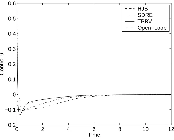
4.3.4 Interpolation of TPBV Problem Solutions . . . 53
4.3.5 Interpolation of Iterative Solutions . . . 55
4.4 Application to Test Problems . . . 57
4.4.1 Example 1: Simple Problem . . . 57
4.4.2 Example 2: Simple Problem . . . 59
4.4.3 Example 3: Larger Flight Dynamics Model . . . 64
4.4.4 Example 4: Flight Model with Quadratic and Cubic Nonlinearities . . . 68
4.5 Conclusions . . . 71
5 State Estimation and Tracking Control of Nonlinear Dynamical Systems 73
5.1 Introduction . . . 73
5.2 The State-Dependent Riccati Equation . . . 75
5.3 Tracking Control for Nonlinear Systems . . . 78
5.4 State Estimation for Nonlinear Systems With Nonlinear Measurements . . . 82
5.5 Application to Test Problems . . . 87
5.5.1 Simple Example System . . . 87
5.5.2 Flight Dynamics Example System . . . 91
5.6 Conclusions . . . 96
6 Surface Flux Tracking With State Estimation 98 6.1 Introduction . . . 98
6.2 Linking the Gas-Phase and Surface Models . . . 98
6.3 Optical Measurement in the HPCVD Reactor . . . 101
6.4 Constructing the Control Problem . . . 103
6.5 Results and Analysis . . . 108
6.6 Conclusions . . . 116
7 Summary and Future Research Directions 119
List of References 122
List of Tables
3.1 Rate constants and activation energies for gas-phase reactions. . . 31
4.1 Numerical comparison of feedback control methodologies in Example 1. . . 59
4.2 Numerical comparison of feedback control methodologies in Example 2. . . 61
4.3 Feedback control methodologies in Example 2 with a distant initial state. . . 62
4.4 Numerical comparison of feedback control methodologies in Example 3. . . 68
4.5 Numerical comparison of feedback control methodologies in Example 4. . . 71
List of Figures
1.1 Photograph of the exterior of the Compact Hard Shell reactor. . . 3
1.2 Photograph of the gas flow channel in the Compact Hard Shell reactor. . . 4
1.3 Outline of the structure of the film growth control problem. . . 6
2.1 The four primary regions involved in thin film deposition. . . 8
2.2 Setup of the PCBE system for III-V compound growth. . . 10
2.3 Setup of growth monitoring by PRS, LLS, and quadrupole mass spectroscopy (QMS). 10 2.4 PRS and LLS monitoring of heteroepitaxial GaP growth under PCBE conditions. . . 11
2.5 PR75 response to periodic TBP and TEG precursor pulses. . . 12
2.6 PR75 responses for various TEG positions within the cycle sequence. . . 13
2.7 PRS and LLS responses to various TEG flow rates (changing at marked positions). . 14
2.8 Extraction of reflectance envelope from PR75 data by removing fine structure. . . . 18
2.9 Simulated PR75 responses for various TEG positions within the cycle sequence. . . . 20
2.10 Properties of the PR75 responses as affected by the TEG start position. . . 21
2.11 Simulated and experimental PR75 first derivatives and reflectances. . . 22
2.12 Simulated and experimental PR75 responses for various TEG flow rates. . . 23
2.13 Construction in the model of simulated reflectance from a source pulse cycle. . . 24
3.1 Three-dimensional view of the HPCVD reactor. . . 29
3.2 HPCVD reactor side-view cross-section (not to scale). . . 30
4.1 Comparison of the norms of feedback controlled trajectories in Example 1. . . 58
4.2 Comparison of the norms of feedback controls in Example 1. . . 59
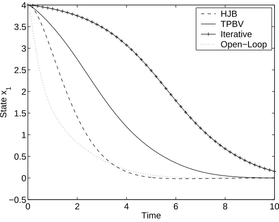
4.3 Comparison of feedback controlled statesx1 in Example 2. . . 60
4.4 Comparison of feedback controls in Example 2. . . 61
4.5 Feedback controlled statesx1 in Example 2 with a distant initial state. . . 63
4.6 Feedback controls in Example 2 with a distant initial state. . . 63
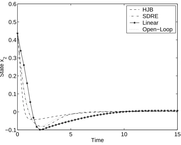
4.7 Comparison of feedback controlled statesx2 in Example 3. . . 66
4.8 Comparison of the norms of feedback controlled trajectories in Example 3. . . 66
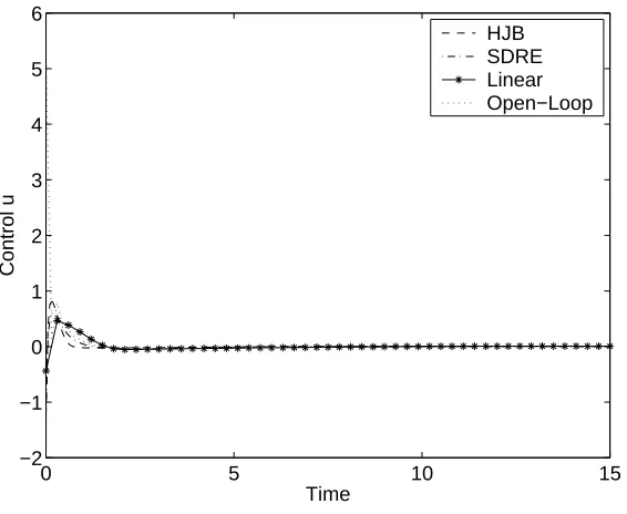
4.9 Comparison of feedback controls in Example 3. . . 67
4.10 Comparison of feedback controlled states x1 in Example 4. . . 70
4.11 Comparison of feedback controls in Example 4. . . 70
5.1 Comparison of feedback tracking controls on Example 1, with weight Q=10. . . 88
5.2 Comparison of feedback tracking controls on Example 1, with weight Q=100. . . 88
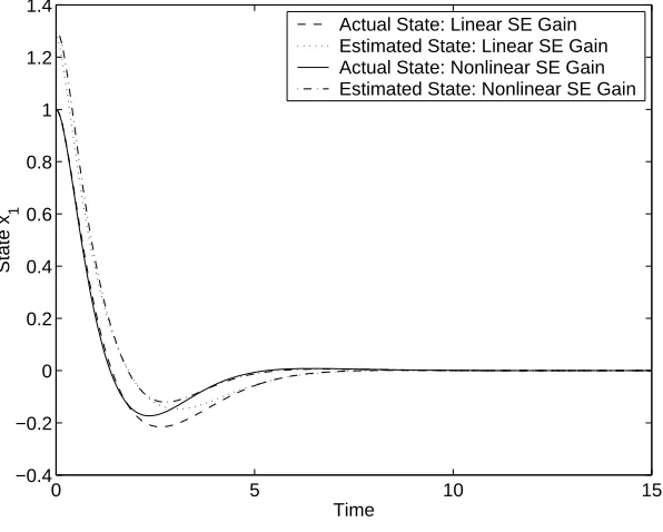
5.3 Actual and estimated states for feedback controls/state estimators in Example 1. . . 89
5.4 Actual and estimated states for nonlinear tracking control/estimator in Example 1. . 90
5.5 Comparison of tracking controls/state estimators on Example 1, with bad (xe)0. . . 91
5.6 Comparison of tracking controls/state estimators on Example 1, with noise. . . 92
5.7 Actual and estimated states for feedback controls/state estimators in Example 2. . . 93
5.8 Comparison of feedback tracking controls on Example 2. . . 94
5.9 Actual and estimated states for nonlinear tracking control/estimator in Example 2. . 94
5.10 Comparison of tracking controls/state estimators on Example 2, with bad (xe)0. . . 95
5.11 Comparison of tracking controls/state estimators on Example 2, with noise. . . 96
6.1 Measurement techniques in the HPCVD reactor. . . 101
6.2 Desired film thickness growth profile. . . 104
6.3 Data variability contained in the first few POD modes, for each species. . . 108
6.4 Controlled thickness profiles for variousr1values. . . 111
6.5 Control inputs for variousr1values, with not-to-scale tracking profile shown. . . 111
6.6 State estimation error amounts for variousr1values. . . 112
6.7 Controlled thickness profiles with sharper target profile. . . 114
6.8 Control inputs with sharper target profile (not-to-scale tracking profile shown). . . . 115
6.9 State estimation error amounts with sharper target profile. . . 115
6.10 Controlled thickness profiles for two r2 values. . . 117
6.11 Control inputs for twor2values (not-to-scale tracking profile shown). . . 117
Chapter 1
Background and Overview
Chemical vapor deposition (CVD) is a technique used to grow very thin films with certain desired
properties, involving the deposition of source vapors onto a heated substrate surface where they
then react chemically to form the desired material. This process is used in the manufacture of
many computer hardware products, including high-speed (GaAs) integrated circuits, transistors,
and DRAM chips, as well as UV detectors and green and blue light emitting diodes. A less
well-known application is in high-performance electrostatic loudspeakers. Precise control of the
film layer thickness and composition is extremely important, and the increasing demands on the
precision of the desired properties make real-time feedback control of the CVD process very desirable
[1, 2, 3, 4]. My research work at North Carolina State University has been in collaboration with
members of the Materials Science, Physics, and Chemical Engineering Departments, as well as the
Mathematics Department, in developing a high-pressure CVD reactor and the real-time sensing and
control techniques to use on the film growth in this reactor.
Low-pressure chemical vapor deposition processes are the preferred choice for manufacturing
many of the devices mentioned above. Previous work within this research group has successfully
implemented feedback control of film thickness and composition in GaP/Ga1−xInxP films, during
experiments in a low-pressure pulsed chemical beam epitaxy (PCBE) reactor using real-time optical
monitoring byp-polarized reflectance spectroscopy (PRS) sensing [4].
However, there are some materials (such as InN or Ga1−xInxN films) which have potential
in-dustrial uses, but cannot be effectively produced at desirable temperatures under low-pressure
con-ditions. Extending the CVD procedure to higher pressures increases our ability to control the
thermal decomposition of certain source gases, and expands the range of compositions which can
be produced at optimal process temperatures. This has applications to flat panel displays covering
Chapter 1. Background and Overview 2
the entire visible wavelength range, and optoelectronics in the visible to UV wavelength range, as
well as radiation-resistant high power electronics. In addition, higher pressures give the advantage
of a fuller ability to intentionally introduce controlled defects into the film or dope the film with
impurities (for example, to give the film a positive charge, in the case of the speaker application).
Control of defect chemistry/residual absorption and laser damage of nonlinear optical materials
(such as ZnGeP2) is also important for wave-guided nonlinear optical sensors and advanced optical parametric oscillators. Higher pressures can also result in faster film deposition and throughput,
an advantage in time-intensive applications in the semiconductor industry. The difficulty in
high-pressure chemical vapor deposition (HPCVD) is that it is significantly more difficult to control than
the low-pressure process, as the higher pressure introduces source vapor gas flow dynamics in the
place of low-pressure ballistic source vapor pulses.
The main focus of the CVD research project at N.C. State is the design and construction of
a HPCVD reactor with real-time sensors to use in feedback control of the film growth process.
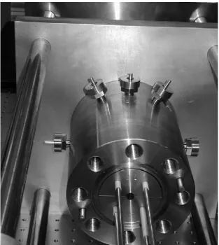
A photograph of this Compact Hard Shell reactor is given in Figure 1.1; it consists of an outer
cylindrical shell around a smaller cylindrical core, which contains a narrow rectangular-box-shaped
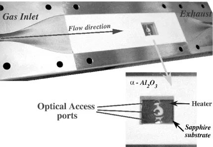
flow channel. A photograph of the flow channel in one of the half-cylinder core parts is shown
in Figure 1.2. The objects seen sticking out of the sides of the cylinder in Figure 1.1 are the
measurement ports for observing the deposition process. The structure of this reactor is described
in more detail in Section 3.2, with a discussion of the measurement techniques in Section 6.3.
In collaboration with the rest of the group, we in the Mathematics Department have worked to
effectively mathematically model the more complicated high-pressure deposition process. Another
aspect of the project is the development of closed-loop control methods to use on the nonlinear
system, including estimation of the state from the sensor measurements and tracking of desired
properties such as film thickness and composition.
One part of the CVD model is the description of the surface kinetics, that is, the decomposition of
source vapors deposited on the surface and their reactions forming the compound which is integrated
into the growing film. These reactions are represented by a reduced order surface kinetics (ROSK)
model which assumes that among the many reactions involved there are a small number of significant
limiting steps. We developed the ROSK model and found values for the unknown parameters
contained in it through comparison of the model with experimental observations of the surface
deposition process at low pressure byp-polarized reflectance spectroscopy (PRS). This model, how
Chapter 1. Background and Overview 3
Figure 1.1: Photograph of the exterior of the Compact Hard Shell reactor.
The second part of the HPCVD process is the gas dynamics present in the high-pressure reactor.
At low pressure the source vapor pulses are assumed to be ballistic beams which travel directly to the
surface, but at high pressure this does not hold. The source vapors travel from the entrance of the
reactor to the surface in a carrier gas at pressures of up to 100 atmospheres and so the mathematical
model describing this process must include the system of partial differential equations representing
the flow dynamics. A dilute approximation is used in our work, leading to a quasi-linear model
with steady-state nonlinear continuity, momentum and energy equations being separated from the
transient linear species equations. When solved numerically by a finite element, finite difference, or
Chapter 1. Background and Overview 4
Figure 1.2: Photograph of the gas flow channel in the Compact Hard Shell reactor.
result in a very large system of ordinary differential equations. This makes real-time model-based
feedback control impossible, so instead we obtain a set of basis functions specific to this problem,
by using the reduced order method known as proper orthogonal decomposition (POD). In earlier
work, members of the N.C. State research group have shown that the POD basis can be used to
represent the species flow dynamics in another HPCVD reactor very efficiently and to compute an
optimal open-loop control [5]. It has also been used to implement feedback control of HPCVD gas
phase species transport to track a desired flux to the surface [6, 7]. Chapter 3 will describe the gas
phase model, including species reactions and boundary conditions, and the use of the POD method
for finding the reduced basis.
The full HPCVD model we will use here includes both the gas phase species transport and the
surface dynamics, with the surface flux from the gas phase linking the two by becoming the source
Chapter 1. Background and Overview 5
on the surface, so a nonlinear feedback control method must be used. Unlike for linear systems,
there is no standard method for feedback control of nonlinear systems. Therefore in Chapter 4 we
compare the performance of several methods from the literature on some simpler test problems, to
gain information with which to choose a particular method to use on the HPCVD problem.
The HPCVD problem also involves more than simple feedback control, however. We want to
track a given film thickness growth curve, so we will need a tracking control instead of a stabilizing
control which simply forces the system to zero. There are also only nonlinear partial measurements
of the growth process available, as will be described in Section 6.3. Lacking full state knowledge, a
state estimator is needed to reconstruct an estimated value of the full state from these measurements.
In Chapter 5 we take one of the nonlinear feedback controls studied in Chapter 4, the state-dependent
Riccati equation (SDRE) method, and extend it into a method for feedback tracking control, as well
as use it in a nonlinear state estimator. These new methods are tested on some simple examples
and their results are compared with those of established linear control methods.
Chapter 6 describes the application of the nonlinear tracking control and state estimation
meth-ods to the combined gas-phase and surface HPCVD model. The goal will be to have the growing
film thickness track a chosen desired profile. This chapter details the linking of the two parts of
the model as well as the formulation of the control problem, including the measurement technique
and the desired tracking signal. Results of the control implementation are given and analyzed, to
study the effectiveness of the POD representation of the species flow, the nonlinear control using it
and the ROSK model, and the state estimation process using an optical absorption measurement for
partial observation of the state. Figure 1.3 shows the structure of this film growth control problem,
the various components of which will be discussed in the following chapters. A summary of all the
research work contained here is given in Chapter 7, with an evaluation of the techniques developed
Chapter 1. Background and Overview 6
Chapter 2
Reduced Order Modeling of the Surface Kinetics
of Thin Film Growth
2.1
Introduction
Understanding and controlling thin film growth is a difficult task, because little is known about
the chemical reaction pathways and reaction kinetics parameters involved in the decomposition of
metalorganic (MO) precursors as source vapors in chemical vapor deposition and their incorporation
into the film. In this chapter these III-V compound/silicon heterostructure growth processes are
described by a reduced order surface kinetics (ROSK) model [8], which reduces the many surface
reactions to a small number of important steps. We will use a series of experiments monitoring
gallium phosphide (GaP) film growth to find estimated values for the unknown constants in the
ROSK model.
To monitor and control the deposition process with stringent tolerances with respect to controlled
thickness and composition of ultrathin layers requires the development of techniques that follow the
deposition process with submonolayer resolution. These demands led to the development of
surface-sensitive real-time optical sensors [9] that are able to move the monitoring and control point close
to the point where the growth occurs, which in a chemical beam epitaxy process is the surface
reaction layer, which is built up by physisorbed and chemisorbed precursor fragments between the
ambient and the film interface. A main challenge in applying optical probe techniques to
real-time characterization of thin film growth is in relating the surface chemistry processes that drive
the growth process to film growth properties, such as composition, instantaneous growth rate or
structural layer quality. As illustrated in Figure 2.1, in deposition four primary regions are involved:
Chapter 2. Reduced Order Modeling of the Surface Kinetics of Thin Film Growth 8
(1) the ambient, (2) the surface reaction layer, which consists of species physisorbed or chemisorbed
to the surface in dynamic equilibrium with both ambient and surface, (3) the surface itself, and (4)
the near-surface region that can be defined as consisting of the outermost several atomic layers of
the fabricated sample. Presently most characterization techniques are aimed towards accurately
Figure 2.1: The four primary regions involved in thin film deposition.
measuring ambient process parameters, such as pressure, flux or temperature. This limits their
ability to deal with complex nonlinear surface chemistry processes, where the surface plays an integral
role in the precursor decomposition pathways and small changes in the ambient composition can
affect the growth substantially. To this end, we have developed and exploredp-polarized reflectance
spectroscopy (PRS) [10, 11, 12] as a highly surface-sensitive monitoring technique, which allows us
to follow the surface reaction kinetics closely under steady-state growth conditions.
To study the ROSK model and try to match its behavior to the actual growth process, we
use PRS-monitored film growth experiments under various conditions. These are pulsed chemical
beam epitaxy (PCBE) experiments done at low pressure, growing GaP heterostructures on Si(001)
substrates. The low-pressure nature of the experiments allows us to focus only on the surface kinetics
without the gas dynamics of the source vapor transport in the high-pressure CVD reactor becoming
a factor. The high surface sensitivity of PRS allows us to follow alterations in the composition and
Chapter 2. Reduced Order Modeling of the Surface Kinetics of Thin Film Growth 9
supply. The linkage of the PRS response to the reduced order surface kinetics model provides the
basis for the estimation of parameters in the ROSK model, and gives insights into the organometallic
precursor decomposition and growth kinetics, allowing us to adjust the model to more accurately
represent the deposition process. The PRS measurement technique has been applied to closed-loop
control of deposition processes at low pressure (PCBE) [8]. A variation on PRS will also be used
as one of the measurements in the physical high-pressure CVD reactor (though not in the model
described here), for real-time observation and control of the film growth.
We will give a brief background on the experimental growth and monitoring conditions in the
PCBE reactor in Section 2.2 and show results obtained by PRS during real-time monitoring of
heteroepitaxial growth of GaP on Si substrates. In Section 2.3 we introduce the model used to
simulate the surface kinetics and the PRS measurements of them. We describe there the link of the
PR response to the simulation parameters within the ROSK model for describing the decomposition
kinetics of the involved organometallic precursors. The process of identifying these parameters
is explained in Section 2.4, and in Section 2.5 the results of the parameter identification through
various experiments are analyzed. In this way we establish and validate surface reaction kinetics
parameters, and advance our understanding of fundamental chemistry processes in thin film growth
using organometallic precursors. We give some concluding remarks on the modeling of CVD surface
kinetics in Section 2.6.
2.2
Experimental Setup and PRS Measurement Results
For monitoring both the bulk and surface properties during heteroepitaxial growth of GaP on Si,
p-polarized reflectance spectroscopy (PRS) has been integrated into a pulsed chemical beam epitaxy
(PCBE) system schematically shown in Figure 2.2. In PCBE, the surface of the substrate is
exposed to pulsed ballistic beams of (C4H9)PH2(tertiary-butyl phosphine, or TBP) and Ga(C2H5)3 (triethylgallium, or TEG) at typically 350−450◦C to accomplish nucleation and overgrowth of the silicon by an epitaxial GaP film. For PRS and laser light scattering (LLS) measurements we employ
p-polarized light beams at two angles of incidence (PR70: φ= 71.5◦ and PR75: φ= 75.2◦) using the wavelength λ = 632.8 nm and Glan-Thompson prisms, as illustrated in Figure 2.3. Further
details on the experimental conditions are given in previous publications [8, 10, 11, 12, 13, 14, 15,
Chapter 2. Reduced Order Modeling of the Surface Kinetics of Thin Film Growth 10
Figure 2.2: Setup of the PCBE system for III-V compound growth.
Chapter 2. Reduced Order Modeling of the Surface Kinetics of Thin Film Growth 11
During the preconditioning period, the PR signals change according to the temperature
depen-dency of the substrate dielectric function. The PR signals are used to verify independent
tempera-ture measurements and to calibrate the actual surface temperatempera-ture. A constant flow of Palladium
purified H2 (10 sccm) is introduced into the growth chamber during the preconditioning as well as
during the growth period. The background pressure in the growth system is<10−9Torr, increasing to 5×10⁻⁵ Torr during pregrowth and to 2×10⁻⁴Torr during growth.
Figure 2.4 shows the PR and LLS signals during heteroepitaxial growth of GaP on Si(001).
A 1200 s preconditioning period begins the observed measurements. After initiating growth at
Figure 2.4: PRS and LLS monitoring of heteroepitaxial GaP growth under PCBE conditions.
1200 s, minima and maxima are observed in the time evolution of the PR signals due to interference
phenomena as the film thickness increases. It should be noted that the maxima and minima of the
two signals are inverted, which is due to the fact that one angle of incidence (PR75) is above – and
the other (PR70) below – the pseudo-Brewster angle of the growing film. Superimposed on the
interference oscillations of the reflectance is a fine structure that is strongly correlated to the time
sequence of the supply of precursors employed during the steady-state growth conditions. The two
insets in Figure 2.4 show enlargements of the fine structure evolutions for 30 s of growth for PR75
and PR70, respectively.
Chapter 2. Reduced Order Modeling of the Surface Kinetics of Thin Film Growth 12
model to be presented in Section 2.3, we varied two experimental parameters: (i) the position of
the TEG pulse of 300 ms length within the precursor cycle sequence and (ii) the TEG flow rate
during the pulse. Each growth condition was carried out and monitored for at least one and a half
interference oscillations in order to get stable steady-state growth and to gather sufficient information
to analyze and compare with simulations of the growth process.
The correlation of the fine structure evolution with the pulsing sequence of the precursor supply
is shown in more detail in Figure 2.5. In this figure the PR75 response is taken during steady-state
Figure 2.5: PR75 response to periodic TBP and TEG precursor pulses.
growth on the rising flank of an interference oscillation, using a pulse cycle sequence of 3 s, a TBP
pulse from 0.0 to 0.8 s, a TEG pulse from 1.3 to 1.6 s and continuous hydrogen flow during the
whole sequence. In the first set of experiments, the flow rates and pulse durations of TBP (800 ms
at 0.907 sccm) and TEG (300 ms at 0.04 sccm) and the start position of the TBP pulse (at 0.0 s)
were kept constant, and only the start position of the TEG pulse was varied, from 0.9 s up to 2.3 s
(increased in steps of 0.2 s). The effect on the fine structure evolution is shown in Figure 2.6, where
the starting point of the TEG pulse is marked by an arrow. This influence of TEG pulse position
on the PR response will be explained more fully in Section 2.5. For comparison, all PR responses
are taken at the same intensity/reflectance level on a rising flank of an interference oscillation. We
Chapter 2. Reduced Order Modeling of the Surface Kinetics of Thin Film Growth 13
Figure 2.6: PR75 responses for various TEG positions within the cycle sequence.
Figure 2.6.
In the second set of experiments, the changes in surface reaction kinetics and growth are evaluated
for TBP:TEG flow ratios between 18 and 30. Figure 2.7 shows the PR and LLS signals during
heteroepitaxial growth of GaP on Si(001) for three TEG flow settings of 0.05, 0.04 and 0.03 sccm
(in a pulse at 1.3-1.6 s), with a TBP pulse of 0.907 sccm at 0.0-0.8 s, in a pulse cycle sequence 3 s in
duration. With decreasing TEG flow, the spacing of the interference oscillations widens according
to the reduced growth rate. More details including comparisons with the results of simulations are
given in Section 2.5.
2.3
Modeling of Surface Reactions and PRS Measurements
We represent the structure of a growing heteroepitaxial film during chemical vapor deposition with
a four-layer medium model consisting of: (1) ambient, (2) surface reaction layer (SRL), (3) film
Chapter 2. Reduced Order Modeling of the Surface Kinetics of Thin Film Growth 14
Figure 2.7: PRS and LLS responses to various TEG flow rates (changing at marked positions).
coefficient forp-polarized incident light, given a four-layer stack, is [23]
rp=
r12(1 +r23r34e−2iβ3) + (r23+r34e−2iβ3)e−2iβ2 (1 +r23r34e−2iβ3) +r12(r23+r34e−2iβ3)e−2iβ2
, (2.1)
where the Fresnel coefficientsrk(k+1) (k= 1, 2, and 3) for the interfaces 1-2, 2-3, and 3-4 are given by [24]
rk(k+1)= k+1
p
k−1sin2φ1−k
p
k+1−1sin2φ1 k+1
p
k−1sin2φ1+k
p
k+1−1sin2φ1
, (2.2)
and the phase shiftsβk for the SRL (k= 2) and the growing film (k= 3) are given by
βk =
2π λ dk
q
k−1sin2φ1. (2.3)
Using equations (2.1)-(2.3), the reflectivity coefficientrp is a function of d2 andd3 (the thicknesses of the SRL and film respectively),1,2,3and4(the complex dielectric functions of the ambient, SRL, film and substrate, respectively), andφ1 andλ. Hereφ1 denotes the angle of incidence and λthe wavelength of the impinging laser light [23].
The values of1,3,4,φ1 andλare constant in time, but2,d2andd3vary in time as the film grows and the SRL composition and thickness change. To understand how these values change, we
need a representative model of the chemical kinetics of the SRL, which approximates the pyrolysis
Chapter 2. Reduced Order Modeling of the Surface Kinetics of Thin Film Growth 15
TEG as source vapors forming GaP, we employ a reduced order surface kinetics (ROSK) model [8].
The ROSK model makes the simplifying assumption that the many reactions which make up the
TBP pyrolysis are combined into one step, the reactions which make up the TEG decomposition
are combined into two steps, and the formation of GaP is one final step. The process is driven by
a periodic source vapor cycle as described in Section 2.2.
Thus the kinetic model representing the reactions in the SRL is given by the following system of
ordinary differential equations:
d
dtn1(t) = S1(t)−k1n1(t)−kGaPn1(t)n3(t)/10
−8mol (2.4)
d
dtn2(t) = S2(t)−k2n2(t)−k3n2(t) (2.5) d
dtn3(t) = k3n2(t)−k4n3(t)−kGaPn1(t)n3(t)/10
−8mol (2.6)
d
dtn4(t) = kGaPn1(t)n3(t)/10
−8mol. (2.7)
The variables n1, n2 and n3 represent the number of moles of the components of the SRL, with n1 being active surface phosphorus fragments, the single stage in the TBP decomposition. An intermediate stage in the TEG decomposition is represented byn2, and we will consider this to be diethylgallium (DEG), whilen3 represents the final stage which we will consider to be monoethyl-gallium (MEG) and active monoethyl-gallium fragments. In equation (2.4) the change in active phosphorus
fragments is written as the sum of a source termS1, a desorption loss term−k1n1, and a nonlinear reaction term forming GaP. The second differential equation, (2.5), which describes the change in
DEG, contains a source term S2, a desorption loss term−k2n2, and a term of decomposition into MEG and active gallium fragments. Equation (2.6) (change in MEG and active surface gallium
fragments) has a term of creation, a desorption loss term, and a reaction term forming GaP. The
variablen4, in equation (2.7), represents the number of moles of created GaP integrated into the de-posited film layer. This equation contains only the single nonlinear reaction term for the formation
of GaP from active surface Ga and P and has to account for any surface activation processes.
The source terms in the differential equations are based on the source vapor pulses. More
specifically, we model the first source term by the following expression:
S1(t) =
P1(t)γβT BP VT BP
, (2.8)
whereP1(t) is the source vapor flow rate. VT BP is the molar volume of TBP and the constantβT BP
Chapter 2. Reduced Order Modeling of the Surface Kinetics of Thin Film Growth 16
vapors actually hit the surface of the Si substrate wafer (a constant dependent on the structure of
the reactor). Similarly, the second source term is represented by
S2(t) =P2(t)γβT EG VT EG
, (2.9)
with correspondingP2(t),VT EG andβT EG for the TEG pulse, and the same constant γ. For each
source term we are using pulsed flow, with a constant flow rate between start and stop times (and
zero flow elsewhere), as described in Section 2.2. There is a small time difference between the
switching on (or off) of the pulse and the start (or stop) of the source vapors at the surface. This is
caused by the time needed for the source vapor gates to open or close and for the vapors to travel to
the surface. We account for it with a parameterdelay, so that for a source vapor pulse set to start
attonand stop attoff, the source vapors will actually reach the surface starting atton+delayand stopping attoff+delay. The delay was estimated to be 0.72 s using the parameter identification process to be described in Section 2.4.
The system of differential equations (2.4)-(2.7), together with the source terms (2.8) and (2.9)
and appropriate initial conditions, can be solved numerically for the number of molesn1,n2,n3and n4 at all times during the growth process. From these solutions, the film and SRL thicknesses are found by the equations
d3(t) = VGaP
A n4(t), (2.10)
d2(t) =
αSRL
A [V1n1(t) +V2n2(t) +V3n3(t)], (2.11)
and the effective dielectric function of the SRL is given by
2(t) = 1 +
"
n1(t)
P3
k=1nk(t) F1+
n2(t)
P3
k=1nk(t) F2+
n3(t)
P3
k=1nk(t) F3
#
, (2.12)
which is derived from the Sellmeier equation [28]. In the above three equations, A is the surface
area of the Si wafer, the valuesVk are the molar volumes of the components nk, and VGaP is the
molar volume of GaP. The parametersFk are the complex optical responses of the components of
the SRL and αSRL is an effective SRL thickness parameter representing the fraction of the SRL
that contributes to the reflectance behavior (as opposed to that which is floating loose on top of the
SRL and does not affect the light beams). With the values of the time-dependent parameters2, d2and d3 found by equations (2.10)- (2.12), and with the constant parameters1, 2, 4, φ1 andλ, the reflectivity coefficientrp can be computed from equations (2.1)-(2.3). From rp, we then find
Chapter 2. Reduced Order Modeling of the Surface Kinetics of Thin Film Growth 17
In the equations described in this section,φ1,λ, 1, V1,V2,V3, VGaP, VT BP,VT EG, A, β1, β2, αSRL, and all start/stop times and flow rates contributing toP1andP2 are known quantities. The values of the dielectric functions3 and 4, the rate constantsk1, k2, k3, k4 and kGaP, the optical
responses F1, F2 and F3, the geometrical parameter γ, and delay are not known. Our work in Sections 2.4 and 2.5 is to find values of these parameters so that the mathematical model most
closely matches experimental results.
2.4
Parameter Identification Problem
Here we formulate the inverse least squares problem used to identify the unknown parameters in
the ROSK model. We want the set of parameters which results in the simulated reflectance (from
the mathematical model described last section) most closely fitting the experimental data.
Specifi-cally, we are looking for the vector of parameters−→q = [F1, F2, F3, k1, k2, k3, k4, kGaP, γ, delay] that
minimizes the cost function
J(−→q) =sX
i
[Rexp(ti)−Rcalc(ti,−→q)]2.
Here Rexp(ti) is the experimental PRS data at the measurement times ti and Rcalc(ti,−→q) is the
simulated data calculated at the same times using the parameter set−→q.
We do not include3 and4in−→q because larger numbers of parameters make the minimization process increasingly difficult. We can remove these two parameters from the above parameter
estimation problem by formulating a separate simpler estimation problem. In particular, we use a
three-layer stack as a simplified model of the growing film, removing the SRL from consideration
and leaving just the ambient, film and substrate layers. The formula for calculating the reflectance
for a three-layer stack analytically is given by
r3,p=
r13+r34e−2iβ3 1 +r13r34e−2iβ3
, (2.13)
wherer13 andr34are the Fresnel coefficients for the reflection from interfaces 1-3 and 3-4 (now that layer 2 is removed), and β3 is the phase shift for the film layer. These values are calculated by formulas analogous to (2.2) and (2.3).
To compare results from this formula with experimental results, we first remove the effects of
the SRL from the experimental data by removing the small-amplitude fine structure oscillations
Chapter 2. Reduced Order Modeling of the Surface Kinetics of Thin Film Growth 18
periodicity of several hundreds of seconds. In order to remove the fine structure, first the curves
on either side of the data forming an envelope around it must be found. The experimental version
of the three-layer stack reflectance is then found by switching from one side of the envelope to the
other where the fine structure ”turns” from positive to negative (from adding to the three-layer stack
reflectance to subtracting from it) or vice versa. This orientation of the fine structure is cyclical
with the interference oscillations, either turning twice per oscillation or else not turning at all, in
which case there is no switching between envelope sides. Figure 2.8 shows this extraction of the
three-layer reflectance out of experimental data near a turning point. The three-layer reflectance
Figure 2.8: Extraction of reflectance envelope from PR75 data by removing fine structure.
plus the minimal influence from the SRL during a cycle is shown on one side of the data (switching
sides at the turning point), while the other side represents the three-layer stack plus the maximal
influence from the SRL during the cycle.
With this method of extracting the experimental three-layer stack reflectance R3,exp, we can
identify the parameters3and4, as well as an average growth rategbr(used to find the film thickness
Chapter 2. Reduced Order Modeling of the Surface Kinetics of Thin Film Growth 19
R3,exp. This is also done through an inverse least squares formulation by finding −→r = [3, 4,bgr]
that minimizes the cost function
J(−→r) =sX
i
[R3,exp(ti)−R3,calc(ti,−→r)]2.
Once the values of3 and4 are found, they can be used in solving the four-layer stack parameter identification problem to find the unknown parameters−→q = [F1, F2, F3, k1, k2, k3, k4, kGaP, γ, delay].
2.5
Analysis of Results
Comparing measurements taken with the TEG pulse position varied while all other conditions are
fixed, as described in Section 2.2 (see e.g., the fine structures shown in Figure 2.6), reveals several
important characteristics in the fine structure. We will explain these features and show how the
mathematical simulation of the growth process, using the reduced order surface kinetics model,
replicates these features.
Looking at the fine structure (in the PR75 data), the most noticeable change with the TEG
pulse position variation is the starting position of the downward slope (near the arrows marked in
Figure 2.6) which is present in every data set but moves to later in the cycle as the TEG pulse moves
to later in the cycle. This start of the downward slope, which is the only feature so dependent on
the TEG pulse placement, clearly relates to the source TEG, the subsequent TEG defragmentation,
and active gallium attachment on the surface.
In contrast, the starting position of the upward slope in the fine structure remains in the same
place shortly after the start of the cycle, independently of the TEG pulse position. It can be related
to the source TBP exposure, its defragmentation, and the formation of active phosphorus on the
surface. Both starting positions are delayed by approximately 0.72 s after the start of the pulses.
This delay is due to the time needed to open the source vapor gates and the time for the vapors to
travel to the surface, as noted in the description of the model in Section 2.3.
The same upward and downward slopes and delay characteristics can be seen in Figure 2.9,
where the fine structure evolutions of the simulated data are compared at the same points as the
experimental data in Figure 2.6, also with the TEG start positions marked by an arrow. The
gap between the downward and upward slopes can be analyzed by the full width at half maximum
(FWHM), defined by the width between the times on the downward and upward slopes with values
Chapter 2. Reduced Order Modeling of the Surface Kinetics of Thin Film Growth 20
Figure 2.9: Simulated PR75 responses for various TEG positions within the cycle sequence.
how this width shrinks as the TEG pulse is moved towards the end of the cycle and closer to the next
TBP pulse. This change, in both the experimental and calculated data, follows the pulse position
nearly linearly.
The fine structure amplitude (the difference between maximum and minimum reflectance over
a cycle) also changes slightly but clearly with the change in TEG pulse position. As shown in
Figure 2.10, the amplitude is largest for TEG pulses near the middle of the range used. This can be
explained as a result of the closeness of the TEG and TBP pulses. If the TEG is input soon after the
TBP, there will be a large GaP formation reaction, leaving little or no active gallium to carry over
to the next cycle. If the TEG comes in very late in the cycle, right before the next TBP pulse, there
may not be time for the decomposition of all the TEG to gallium to occur before the GaP formation
with the incoming phosphorus starts. With a more central TEG pulse, the phosphorus and gallium
will each have the time to build up on the surface, in turn creating more extreme changes in the
SRL thickness and composition and therefore a larger fine structure amplitude.
Chapter 2. Reduced Order Modeling of the Surface Kinetics of Thin Film Growth 21
Figure 2.10: Properties of the PR75 responses as affected by the TEG start position.
fairly high on a rising flank. Other places, particularly on the other side of a turning point, will
have different characteristics (for example, the TEG pulse may result in a jump upward and the
TBP pulse in a jump downward).
One larger-scale feature of the reflectance data we can look at is the average film growth rate
for the various TEG pulse positions, shown in Figure 2.10. The general downward slope can be
explained in terms of the closeness of the two pulses. As the TEG pulse moves later in the cycle
away from the TBP pulse there is less phosphorus to react with, so there is more active gallium left
on the surface to be lost via desorption before the next cycle. The TEG pulse positions nearest the
start of the cycle seem to be too close to the TBP pulse for the fastest growth rate, however. The
incoming TEG and its defragmentation products may be partially blocked from the available active
phosphorus in the SRL by TBP that failed to stick and/or desorbed phosphorus that is sitting loose
on the surface.
Another large-scale characteristic feature of the data sets is the position of (or complete lack
of) turning points in the fine structure. These come in pairs for every interference oscillation or
Chapter 2. Reduced Order Modeling of the Surface Kinetics of Thin Film Growth 22
turning point positions can be characterized by the derivative of the reflectance. The derivative
amplitude is related to the periodic thickness changes in the SRL. This amplitude is minimized at
the turning points, where the fine structure amplitude is smallest and so the reflectance curve is
least steep. Figure 2.11 shows the close match between the experimental and calculated derivative
amplitudes, which characterize the fine structure amplitudes as well as their turning point positions
(using TEG pulse position 1.3-1.6 s). In earlier works [11, 12], we showed that the locations of these
Figure 2.11: Simulated and experimental PR75 first derivatives and reflectances.
turning points change as a function of the SRL dielectric properties. The good agreement shown
in Figure 2.11 indicates that the SRL dielectric properties were obtained correctly. The simulated
PR75 reflectance matches the experimental reflectance shown in 2.11 so closely that with the two
Chapter 2. Reduced Order Modeling of the Surface Kinetics of Thin Film Growth 23
The measurements taken with the TEG pulse position fixed but the flow rate varied (as described
in Section 2.2) also correspond to what the model predicts. Examples of the fine structure (again
for PR75) for the three TEG flow rates are shown in Figure 2.12 for both experimental data and
simulated data. In contrast with the variation of the pulse position, here the shape of the fine
Figure 2.12: Simulated and experimental PR75 responses for various TEG flow rates.
structure remains the same, since the shape of the source vapor cycle is the same. The positions
of changes in the slope remain constant due to the constant position of the TEG pulse. However,
the amplitude of the fine structure does change, since as the TEG flow rate increases there will be
more gallium deposited in the SRL, and this will have a larger effect on the reflectance. Increased
TEG flow also results in a faster film growth rate, which causes steeper large-scale curves as seen
in Figure 2.12 and faster interference oscillations as seen in Figure 2.7. Both the experimental and
simulated data sets show these characteristics, and they agree with each other extremely well.
The steps in the generation of a set of simulated data which was used to compare with the
experimental data presented in Figure 2.4 are shown in detail in Figure 2.13 for a TEG pulse of
Chapter 2. Reduced Order Modeling of the Surface Kinetics of Thin Film Growth 24
Figure 2.13: Construction in the model of simulated reflectance from a source pulse cycle.
the result of the source pulses and the ROSK model simulation. From the SRL components, the
SRL thickness and dielectric function are found. These values then contribute to the calculated
reflectance. Figure 2.13 shows how the arrival of gallium in the SRL causes the downward slope in
the fine structure and how the arrival of phosphorus causes the upward slope. The good fit of this
simulated fine structure to the experimental data as shown in Figure 2.13 will also hold for the rest
of the interference oscillations. This is illustrated in Figure 2.11, where the reflectance curves and
reflectance derivatives match (and the fine structure amplitudes and turning points agree as well).
The closeness of the fit and the correlation of the significant features discussed above support the
Chapter 2. Reduced Order Modeling of the Surface Kinetics of Thin Film Growth 25
An important aspect of the behavior of the SRL kinetics which can be seen in Figure 2.13 is the
difference between a phosphorus-terminated and gallium-terminated surface at the end of a cycle
sequence. We had originally expected a phosphorus-terminated surface at the end of each 3 s cycle,
where the TEG pulse is almost completely used up through desorption or formation of GaP, leaving
some phosphorus in the SRL at the start of the next pulse cycle. However, simulated reflectance
data with this type of behavior could not fit the experimental data. Instead, a set of parameters
which resulted in a gallium-terminated surface (where the TEG pulse is not all used up at the end
of the cycle time, leaving an amount of gallium in the SRL being carried over to the next cycle)
gave a much more accurate fit as described above.
The data sets measured at the second angle (PR70) have structures and features similar to the
PR75 data, with the major difference being the inversion of interference oscillation maxima/minima
since the angles are on opposite sides of the pseudo-Brewster angle. Analysis of these measurements
using the same model results in parameters similar to those found for PR75 (which are given below)
and a similar fit of the reflectance data. There are a few noticeable differences between the two,
which can be explained by the measurements being taken with light beams hitting different points
on the surface. If the growth is somewhat uneven this could cause differences in the parameters in
the growth model when the two data sets are compared.
The values used in the calculations of the model are as follows. The molar volumes used in
the minimization process areVT BP = 128.6 cm3/mol, VT EG = 148 cm3/mol, V1 = 17 cm3/mol, V2 = 13 cm3/mol,V3 = 11.8 cm3/mol, andVGaP = 12.2 cm3/mol. The sticking coefficients used
are βT BP = 0.15 andβT EG = 1.0, the effective SRL thickness parameter isαSRL = 0.75, and the
substrate is a 2-inch diameter circular wafer. The geometrical parameterγ= 0.025 was estimated
in the minimization process.
The numerical simulations were implemented using programs written in MATLAB code. The
differential equations were solved numerically by the built-in function ”ode23”, an adaptive mesh
and low order Runge-Kutta method. The optimization problems were solved using either a
Nelder-Mead algorithm [29, 30, 31] or a Hooke-Jeeves procedure [29]. We are grateful to Professor C. T.
Kelley for providing us with the code ”nelder” implementing the Nelder-Mead algorithm and to
Mr. D. Bortz for providing us with the code ”hj” implementing the Hooke-Jeeves procedure. Both
Professor Kelley and Mr. Bortz are in the Department of Mathematics at N.C. State.
We estimated the following parameters by averaging the results of independent best fits of the
Chapter 2. Reduced Order Modeling of the Surface Kinetics of Thin Film Growth 26
stack problem resulted in 3 = 10.60−0.06i and 4 = 15.82−0.27i. With these, the parameter estimation using the four-layer stack model gave the following parameter values: rate constants
of k1 = 3.31 s−1, k2 = 1.55 s−1, k3 = 2.14 s−1, k4 = 0.052 s−1, and kGaP = 2.0 s−1, and optical
responses of F1 = 13.46−0.13i, F2 = 13.56−0.0i and F3 = 19.36−11.02i. An earlier study on the decomposition kinetics of TEG, analyzing the PR responses to TEG exposure after growth
interruptions [17], gave rate constants of k3 = 0.4 s−1 andkGaP = 0.24 s−1. The higher value for kGaP here was expected since no thermally activated hydrogen was employed to the growth surface
and the flow rates were lower by a factor of about 2 in our experiments.
2.6
Conclusions
In this chapter we introduced a reduced order surface kinetics model using generalized reaction
rate parameters to describe the decomposition kinetics of the organometallic precursor species TBP
and TEG in heteroepitaxial growth of a gallium phosphide film on a silicon substrate. The set of
coupled differential equations that describe the surface reaction kinetics provide information about
the dynamics of molar concentrations of precursor fragments stored in the surface reaction layer
and their incorporation into the underlying growing film. We fitted sets of low-pressure PCBE
experimental data using the ROSK model to identify the unknown parameters involved in the
surface kinetics and study their effects on the PR measurements. The results showed that the
mathematical model can be used to effectively represent the deposition process and predict the
large-scale and small-scale features of the experimental data. A true experimental validation of the
ROSK model’s predicted surface reaction layer constituents and their concentrations will require the
development of highly surface sensitive, molecular specific diagnostic techniques that allow analysis
of the dynamics in the SRL under steady-state growth. For this, the application of PRS in the
infrared wavelength regime, using tuneable laser sources, has been proposed. To extend the chemical
vapor deposition model to the high-pressure case, we will need to add the gas-phase species transport
Chapter 3
Reduced Order Modeling of Gas-Phase Species
Transport
3.1
Introduction
This chapter will present the gas-phase flow model of the high-pressure chemical vapor deposition
reactor, largely based on the previous work by other members of the N.C. State research group in
[6, 7]. These papers construct mathematical models with which to simulate and control the flow of
precursor species from the inlet to the substrate surface. We will be coupling a version of this
gas-phase model, described below, with the reduced order surface kinetics model discussed in Chapter 2
to create a model representing the whole HPCVD process from inlet flow to reactions causing film
growth (this linkage is done in Section 6.2). The species transport process dynamics are given by
the partial differential equations for continuity, momentum, energy and species balances, including
multiple species and gas-phase reactions [32, 33, 34, 35]. The formulation is quasi-steady, with
steady-state continuity, momentum and energy equations, and transient species equations. These
general equations representing the reactor transport dynamics are discussed in Section 3.2. A generic
numerical simulation of the time-dependent species equations using a standard finite element, finite
difference or spectral method would lead to a system of ordinary differential equations far too large
to be used for model-based real-time feedback control. Thus we use instead the proper orthogonal
decomposition (POD) reduced basis method to limit the number of equations necessary, making
the implementation of model-based feedback control possible. The POD method finds a set of
basis functions which incorporate the dynamics of the particular problem (here the HPCVD species
transport) and thus can represent the problem using very few basis functions compared with more
Chapter 3. Reduced Order Modeling of Gas-Phase Species Transport 28
general methods. The POD itself and its properties are described in Section 3.3, while the use of
the POD basis in a Galerkin formulation to obtain the reduced order ODE system is the subject of
Section 3.4. Section 3.5 gives some overall conclusions on the gas-phase modeling process.
3.2
Transport Equations
The gas dynamics equations are considered for a case with only trace amounts of the precursors
mixed with the carrier gas (N2). With this dilute assumption the continuity, momentum and
energy equations can be solved as steady-state equations, based on the properties of the dominant
carrier gas and independent of the reactant concentrations:
−
→∇ ·(ρ−→v) = 0 (3.1)
ρ−→v · −→∇−→v = −−→∇P+−→∇ · −→τ −ρ−→g (3.2)
ρcp−→v · −→∇T = →−∇ ·(k−→∇T), (3.3)
where the viscous stress tensor is given by
− →τ =−2
3µ(
−
→∇ · −→v)−→I +µ(−→∇−→v +−→∇−→vT). (3.4)
Here −→v, T andP are the velocity, temperature and pressure,−→g is the gravitational acceleration,
and µ, cp and k are the viscosity, specific heat and conductivity of the carrier gas. The density
variation is modeled as
ρ=ρ0[1−β(T−T0)], (3.5)
with a reference temperature T0, a reference density ρ0 calculated from the ideal gas law at the reference temperature and reactor pressure, and the volume coefficient of expansionβ= 1/T.
We will consider a three-dimensional rectangular-box-shaped domain describing the reactor
de-picted in Figure 3.1. Previous work [6, 7] used a two-dimensional representation of an earlier
HPCVD reactor, but all three dimensions are necessary for this model, because in addition to the
predominantly lengthwise gas flow and vertical deposition there is now also a horizontal measurement
of optical absorption across the width of the reactor (to be discussed in Section 6.3). Our numerical
model will represent an area of this reactor that is 150 mm long, 50 mm wide, and only 1 mm high.
A side-view cross-section of this is shown in Figure 3.2, with the very small height not to scale. The
portions of the reactor outside this domain, specifically the narrow inflow and outflow regions and
Chapter 3. Reduced Order Modeling of Gas-Phase Species Transport 29
Figure 3.1: Three-dimensional view of the HPCVD reactor.
There are two substrates on which the growth is to take place, each 25 mm long by 20 mm wide and
placed in the center of the reactor model (width-wise and length-wise), located symmetrically on
both the top and bottom of the flow channel. The growth is driven thermally by a circular heating
element, or susceptor, 40 mm in diameter and centered behind each substrate. The substrate and
heating element placement can be seen in Figures 3.1 and 3.2, as well as in the photograph of the
physical reactor flow channel in Figure 1.2. The optical access ports noted in Figure 3.1 in the
heater beneath the substrate are for a variation on the PRS monitoring technique. This will be
used in the physical reactor as a second measurement of the system, but our model will only involve
the optical absorption measurement described in Section 6.3. The gas flow enters through the inlet
seen at the left end of the reactor in these figures, flows across the substrate surfaces (depositing
some of the gallium species there), and exits the outlet at the right end of the reactor. Here we
consider Nitrogen (N2) as the carrier gas, at a pressure of 10 atmospheres. Temperature-dependent
Chapter 3. Reduced Order Modeling of Gas-Phase Species Transport 30
Figure 3.2: HPCVD reactor side-view cross-section (not to scale).
is a no-slip (zero velocity) condition on all walls of the reactor, as well as the substrate, while the
inflow velocity profile corresponds to rectangular duct flow [39] with a flow rate of 10 standard liters
per minute (slpm). The temperature boundary condition is room temperature (298 K) at the inlet
and 1000 K at the heaters. Boundary conditions on the temperature at the rest of the reactor walls
include conduction from the heaters along the walls, radiation off of the surfaces, convective heat
loss to the environment, and modeled heat loss to the outside of the reactor. A special boundary
condition in the FIDAP package, described in [34], page 6-14, is used to obtain a smooth outflow
condition. The pressure is involved in equations (3.1)-(3.5) only as−→∇P, so therefore only pressure
differences matter, not absolute values, and an implicit P = 0 boundary condition is used at the
outlet. A Galerkin finite element method with weighted residuals for the degrees of freedom (−→v,T
andP) is used to discretize the gas flow equations. The discretization uses a mixed formulation with
4983 brick elements (corresponding to 47131 nodes), with piecewise linear discontinuous elements
for pressure and quadratic (27-noded) elements for the other degrees of freedom. The commercial
software package FIDAP was used to solve the finite element problem for values of−→v, T andP at
the nodal points.
The solutions for velocity, temperature and density that are found from equations (3.1)-(3.5)
can then be used in the solution of the time-dependent species equations for the precursor mass
fractions,
∂Yn
∂t +−→v · −
→∇Y n =
1 ρ
− →∇ ·(ρD
n−→∇Yn) + NR
X
i=1
rni, (3.6)
whereYn is the mass fraction of thenth species,Dnis the diffusivity of speciesn,NRis the number
of gas phase reactions, andrniis the rate of production of speciesnin theith reaction.
Chapter 3. Reduced Order Modeling of Gas-Phase Species Transport 31
and phosphine (PH3) as source materials for the growth of the III-V film gallium phosphide (GaP).
For now we only look at the TMG pulse, in terms of representing it by POD modes and using
those to control its contribution to the film deposition. This can be done because of the pulsing
of the inputs with pauses in between, so that the gallium species and phosphorus species are not
present in the reactor at the same time (though a constant overall gas flow profile is maintained
throughout the pulsing cycle by the carrier gas). This pulsing prevents nucleation of the film in
the gas phase. For the gallium transport we will consider three gas-phase species (aside from the
carrier gas): Y1 representing the mass fraction of TMG,Y2 that of dimethylgallium (DMG), and Y3that of monomethylgallium (MMG).
We will assume that there areNR= 2 significant gas phase reaction mechanisms for the gallium
species. There is the reaction for the decomposition of TMG to DMG and a methyl molecule,
Ga(CH3)3 →Ga(CH3)2 + CH3, and the decomposition of DMG to MMG and a methyl molecule,
Ga(CH3)2 → GaCH3 + CH3. These decompositions can be described as first-order Arrhenius
reactions with rates of production given by
rni=νni Wn Wmi
kie−Ei/RTYmi, (3.7)
where mi is the number of the species which is the source in reactioni. The parameterνni is the
stoichiometric constant for speciesnin reactioni, Wn andWmi are the molecular weights of those particular species, andkiis the rate constant andEithe activation energy for reactioni. The values
ofνni,ki andEifor the two reactions we consider are taken from [40, 41] and are given in Table 3.1.
The molar weights for the three species are WT M G = 114.8 g/mol, WDM G = 99.79 g/mol, and
Reactioni Speciesn νniki (s−1) Ei(kcal/mol)
1 1 (m1) −5.5×10¹⁵ 61.0
1 2 5.5×10¹⁵ 61.0
2 2 (m2) −8.7×10⁷ 35.4
2 3 8.7×10⁷ 35.4
Table 3.1: Rate constants and activation energies for gas-phase reactions.
WM M G= 84.755 g/mol, andR= 1.99 cal/(mol·K) is the universal gas constant. The temperature
dependent values of the diffusivitiesDn are linearly interpolated from values in the literature [42].
The methyl molecules do not participate in the film growth and, due to the dilute approximation,
Chapter 3. Reduced Order Modeling of Gas-Phase Species Transport 32
The boundary conditions for the species transport equations will be as follows. We consider
the substrate, as well as the parts of the reactor walls directly above the heated susceptor, to be
perfectly absorbing, and the other walls completely non-absorbing, for each species. At the inlet,
the source species (TMG) is set to desired values, and will be used as the input for control of the
growth process, while the other two species are set to 0. Zero normal flux is assumed at the outflow,
so that ∂Yn/∂−→n = 0. The initial condition of the system is that no species are present in the
reactor. Thus the entire time-dependent species transport system based on equation (3.6) is given
by
∂Yn
∂t +−→v · −
→∇Y
n =
1 ρ
− →∇ ·(ρD
n−→∇Yn) + NR
X
i=1 rni
Yn(0,−→x) = 0
Y1(t,−→x) = u1 at inflow (3.8)
Yn(t,−→x) = 0 at inflow (n= 2,3)
Yn(t,−→x) = 0 at substrate, susceptor ∂Yn(t,−→x)
∂−→n = 0 at walls, outflow,
where rni are the reaction production rates from equation (3.7) andu1 is the control input which will be discussed later.
We use a penalty boundary formulation on the species transport problem in order to change
all the boundary conditions to Neumann conditions. This prepares the system for the Galerkin
procedure to be discussed in Section 3.4 and the control problem to be described in Chapter 6.
Under the penalty boundary formulation the system (3.8) is modified to become
∂Yn
∂t +−→v · −
→∇Y
n =
1 ρ
− →∇ ·(ρD
n−→∇Yn) + NR
X
i=1 rni
Yn(0,−→x) = 0 ∂Y1(t,−→x)
∂−→n = 1
(Y1(t,−→x)−u1) at inflow (3.9) ∂Yn(t,−→x)
∂−→n = 1
Yn(t,−→x) at inflow (n= 2,3) ∂Yn(t,−→x)
∂−→n = 1
Yn(t,−→x) at substrate, susceptor ∂Yn(t,−→x)
∂−→n = 0 at walls, outflow,