Modeling and Control: Applications to a Double Inverted Pendulum and Radio Frequency Interference.

ABSTRACT

BERNSTEIN, AMANDA SUE. Modeling and Control: Applications to a Double Inverted Pendulum and Radio Frequency Interference. (Under the direction of Hien Tran).

In this work we consider methods for the modeling and control of physical systems. In particular, we examine a double inverted pendulum (DIP) system and the impact of radio frequency interference (RFI) on satellite operations (SATOPS) systems.

The DIP is a classic example of a nonlinear, multivariable, unstable system. For the stabi-lization problem, a controller is designed that stabilizes the pendulum system in the unstable equilibrium position. Physically, this is the position where the two pendulum rods are aligned in a vertical position. The mathematical model of the DIP is derived using Lagrange’s energy method, and parameter estimation is performed to optimize the friction parameters. The result-ing nonlinear system is linearized about its unstable equilibrium state, and a linear quadratic regulator (LQR) control and a power series based nonlinear control are each implemented in real-time in order to stabilize the DIP system. Since the real-time system only measures the three position states of the system, the three velocity states must also be estimated in order to apply the state feedback controls. Thus, three estimation methods are presented: a low pass derivative filter, a Kalman observer, and a nonlinear observer. Only the low pass derivative filter is successful in estimating the velocity states and is thus used to obtain the real-time results.

© Copyright 2018 by Amanda Sue Bernstein

Modeling and Control: Applications to a Double Inverted Pendulum and Radio Frequency Interference

by

Amanda Sue Bernstein

A dissertation submitted to the Graduate Faculty of North Carolina State University

in partial fulfillment of the requirements for the Degree of

Doctor of Philosophy

Applied Mathematics

Raleigh, North Carolina

2018

APPROVED BY:

Stephen Campbell Negash Medhin

Tien Khai Nguyen Hien Tran

DEDICATION

BIOGRAPHY

ACKNOWLEDGEMENTS

I would like to thank my advisor, Dr. Hien Tran, for all his support and guidance as I worked on this research. Thank you also to our collaborator, Dr. Tien Nguyen, for his contributions to this research. I also thank my committee members, Dr. Stephen Campbell, Dr. Negash Medhin, and Dr. Khai Nguyen, for their time and feedback.

Thank you to the NCSU Mathematics Department and the CRSC for their financial support throughout my time here at NC State.

TABLE OF CONTENTS

LIST OF TABLES . . . vii

LIST OF FIGURES . . . .viii

Chapter 1 Introduction . . . 1

1.1 The Double Inverted Pendulum . . . 1

1.2 Radio Frequency Interference Modeling . . . 4

1.3 Thesis Outline . . . 5

Chapter 2 Modeling of an Inverted Double Pendulum System . . . 6

2.1 Frame of Reference . . . 6

2.2 Equations of Motion . . . 7

2.2.1 Potential Energy . . . 9

2.2.2 Kinetic Energy . . . 9

2.2.3 Lagrange’s Equations . . . 11

2.2.4 Converting to Voltage Input . . . 14

2.3 Model Calibration . . . 15

Chapter 3 Stabilization Control of an Inverted Double Pendulum System . . . 21

3.1 Overview of Existing Control Methods . . . 21

3.2 Problem Statement . . . 23

3.3 LQR Control . . . 24

3.3.1 An Application Example . . . 26

3.4 Nonlinear Control . . . 28

3.4.1 Power Series Based Controller . . . 29

3.4.2 An Application Example . . . 30

3.5 Simulation Results . . . 31

3.6 Experimental Results . . . 33

3.6.1 Experimental Apparatus . . . 33

3.6.2 Experimental Procedure . . . 33

3.6.3 Results for the LQR Controller . . . 35

3.6.4 Results for the Power Series Controller . . . 38

Chapter 4 State Observation for an Inverted Double Pendulum System . . . . 43

4.1 Low Pass Derivative Filter . . . 44

4.2 Kalman Observer . . . 45

4.2.1 An Application Example . . . 49

4.2.2 Application to the DIP System . . . 53

4.3 Nonlinear Observer . . . 53

4.3.1 An Application Example . . . 57

4.3.2 Application to the DIP System . . . 60

4.3.2.1 The Complex Step Method . . . 60

4.4 Summary of the Observer Used for the DIP System . . . 64

Chapter 5 Modeling of Radio Frequency Interference for SATOPS Applications 65 5.1 Background . . . 65

5.1.1 The RFI Detection Problem . . . 67

5.1.2 The RFI Prediction Problem . . . 67

5.1.3 Existing RFI Tools . . . 69

5.2 RFI Analytical Models for Acquisition Time . . . 69

5.2.1 Carrier Frequency Acquisition Mode . . . 69

5.2.2 Carrier Phase Acquisition Mode . . . 70

5.2.2.1 Sync Word Technique . . . 71

5.2.2.2 Phase Sweeping Technique . . . 71

5.2.3 PLL Acquisition in the Presence of CW RFI . . . 72

5.2.4 PLL Acquisition in the Presence of WB RFI . . . 73

5.2.5 Simulation Results for Verification and Validation . . . 74

5.3 Analytical Models for RFI Detection . . . 77

5.3.1 The PLL Lock Detector . . . 77

5.3.2 PLL Tracking Jitter in the Absence of RFI . . . 80

5.3.3 PLL Tracking Jitter in the Presence of CW RFI . . . 81

5.3.4 PLL Tracking Jitter in the Presence of WB RFI . . . 82

5.3.5 Simulation Results for Verification and Validation . . . 82

Chapter 6 Conclusion . . . 86

6.1 The Double Inverted Pendulum System . . . 86

6.2 Radio Frequency Interference Analytic Models . . . 87

REFERENCES . . . 88

APPENDIX . . . 92

Appendix A DIP Model Parameters . . . 93

A.1 Nomenclature . . . 93

LIST OF TABLES

Table 2.1 Optimized friction parameter values found using fminsearch. . . 18

Table 3.1 Maximum and average values for the states and control voltages using the LQR controller with various values of Q and R. (xc[mm], α[degrees],

θ[degrees],Vm[V]). . . 38

Table 3.2 Maximum and average values for the states and control voltages using the power series based controller with various values of Q and R. (xc[mm],

α[degrees],θ[degrees],Vm[V]). . . 41

Table 5.1 Parameters for the simulations of PLL acquisition performance: Carrier acquisition time. . . 74 Table 5.2 Parameters for the simulations of PLL acquisition performance: Tracking

error and BER. . . 83

LIST OF FIGURES

Figure 1.1 Some applications of the double inverted pendulum: (a) a robot arm and

(b) a gymnast. . . 2

Figure 1.2 The double inverted pendulum mounted on a cart. . . 3

Figure 1.3 A typical satellite control network (SCN). . . 4

Figure 2.1 Free body diagram of the DIP system mounted on a cart. . . 7

Figure 2.2 Electrical schematic of a standard DC motor. . . 14

Figure 2.3 Input voltage for use in model calibration. . . 16

Figure 2.4 Experimental and model simulation results using the parameter values provided by Quanser. . . 17

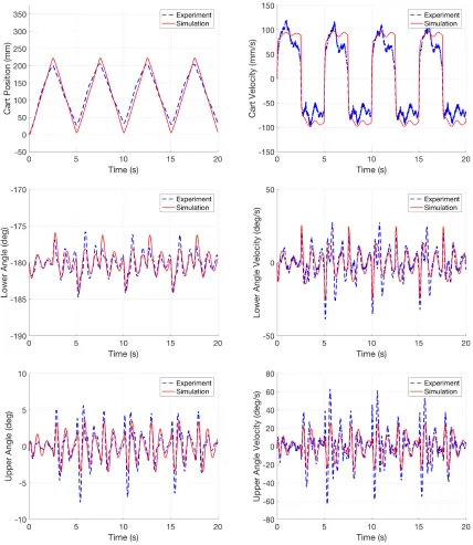
Figure 2.5 Experimental and model simulation results using the optimized friction parameter values. . . 19

Figure 2.6 Residuals between the experimental and model simulation results using the optimized friction parameter values. . . 20

Figure 3.1 LQR control applied to example problem: (a) state trajectories and (b) control effort. . . 28

Figure 3.2 Power series based control applied to example problem: (a) state trajec-tories and (b) control effort. . . 31

Figure 3.3 Simulation results for the state trajectories using the LQR controller with Q= diag(30,350,100,0,0,0) and R= 0.1. . . 32

Figure 3.4 Control effort for the simulation using the LQR controller with Q = diag(30,350,100,0,0,0) and R= 0.1. . . 33

Figure 3.5 A diagram of the experimental setup for the DIP system. . . 34

Figure 3.6 Simulink block diagram governing the real-time implementation of the DIP system. . . 34

Figure 3.7 Real-time experimental results for the state trajectories using the LQR controller with Q= diag(30,350,100,0,0,0) and R= 0.1. . . 36

Figure 3.8 Control effort for the real-time experiment using the LQR controller with Q= diag(30,350,100,0,0,0) and R= 0.1. . . 37

Figure 3.9 Real-time experimental results for the state trajectories using the power series based controller with Q= diag(30,350,100,0,0,0) and R= 0.1. . . 39

Figure 3.10 Control effort for the real-time experiment using the power series based controller with Q= diag(30,350,100,0,0,0) and R= 0.1. . . 40

Figure 4.1 Diagrammatic representation of the state observer problem. . . 43

Figure 4.2 The Kalman observer applied to the example problem using the power series based control: (a) x1 and (b)x2. . . 50

Figure 4.3 Absolute error between the observer and system state values for the ex-ample problem using the Kalman observer. . . 51

Figure 4.5 Absolute error between the observer and system state values for the

ex-ample problem using the Kalman observer including white noise. . . 52

Figure 4.6 Simulation results for the states of the observer and the linearized DIP system using the Kalman observer and the power series based controller. . 54

Figure 4.7 Control effort for the simulation using the Kalman observer and the power series based controller. . . 55

Figure 4.8 A one-link robot arm. . . 58

Figure 4.9 System and observer performance for the one-link robot arm. . . 61

Figure 5.1 Typical RFI scenarios involving friendly sources. . . 66

Figure 5.2 Interference bandwidth for evaluating potential RFI events and the cor-responding CCI and ACI scenarios. . . 66

Figure 5.3 A general block diagram of a PLL. . . 68

Figure 5.4 Carrier acquisition times vs. loop SNR without RFI and with CW RFI at ISR = -40 dB. . . 75

Figure 5.5 Carrier acquisition times vs. loop SNR without RFI and with CW RFI at ISR = -25 dB. . . 76

Figure 5.6 Carrier acquisition times vs. loop SNR without RFI and with WB RFI at ISR = -40 dB. . . 77

Figure 5.7 Carrier acquisition times vs. loop SNR without RFI and with WB RFI at ISR = -25 dB. . . 78

Figure 5.8 A typical PLL lock detector used by SATOPS satellites. . . 79

Figure 5.9 PLL tracking jitters in the absence of RFI and the presence of CW and WB RFI signals with ∆fRF I = 5 Hz. . . 83

Figure 5.10 PLL tracking jitters in the absence of RFI and the presence of CW and WB RFI signals with ∆fRF I = 10 Hz. . . 84

Figure 5.11 BER in the absence of RFI and the presence of CW and WB RFI signals with ∆fRF I = 5 Hz. (b) shows detail on the BER in the presence of CW and WB RFI. . . 85

Chapter 1

Introduction

Mankind has always sought to understand our universe and to control it for our own aims. As mathematicians, one of the ways we seek to understand is by creating models. Whether we are looking to comprehend the ups and downs of the stock market, the spread of pathogens through a population, or how a self-driving car operates, models can give us insight to these systems and allow us to predict what will happen in the future. Furthermore, by including control variables in our models, we can change the outputs to suit our desires. Models can take many forms, but most commonly we use systems of equations to represent them as well as to describe the ways we want to control them. In this thesis, we will examine the models of two different systems, a double inverted pendulum and radio frequency interference within a satellite operations system, as well as ways to control the double inverted pendulum system.

1.1

The Double Inverted Pendulum

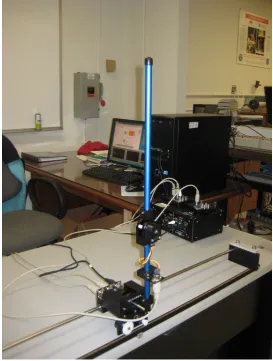
For this work, we will consider the double inverted pendulum (DIP) system mounted on a cart. This is an extension of the single inverted pendulum with an additional pendulum rod attached via a hinge. Imagine you break your broomstick into two pieces, reattach them using a hinge, and now balance that on your open palm. DIP systems can be used as models for a number of different applications, including self-stabilizing robots and robotic limbs [34, 36], human posture, and gymnast motion [38]. Currently, the DIP is used as a model for human standing where the pivot of the pendulum is the ankle joint and the hinge is the hip joint with the legs and the torso comprising the two pendulum rods [35, 39]. Some of these applications are shown in Figure 1.1.

(a) (b)

Figure 1.1: Some applications of the double inverted pendulum: (a) a robot arm and (b) a gymnast.

provide real-time experimental implementation on a physical system.

For our work, we use an apparatus of the DIP system which was provided by Quanser Consulting, Inc. (119 Spy Court, Markham, Ontario, L3R 5H6, Canada). This system is depicted in Figure 1.2. The DIP system consists of two aluminum rods, one 12 inches long and one 7

Figure 1.2: The double inverted pendulum mounted on a cart.

to compute this voltage will be one of the focuses of this work.

1.2

Radio Frequency Interference Modeling

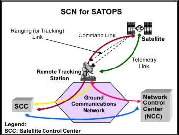
Satellite operations (SATOPS) services are provided by a satellite control network (SCN) and include capabilities to provide tracking, telemetry, and command services [26]. Figure 1.3 shows an example of what a satellite control network may consist of. The ground tracking station

Figure 1.3: A typical satellite control network (SCN).

SATOPS typically operate in L-band (1–2 GHz) or S-band (2–4 GHz) frequencies where there are many potential sources for radio frequency interference (RFI) [25, 28, 29]. RFI oc-curs when the victim receiver simultaneously collects power from its desired signal as well as other undesired interfering signals. Depending on the power of the interfering signals, this can degrade the system performance and could result in data blockages. These frequency bands are shared by many systems, ranging from the Global Positioning System (GPS) to wireless mobile communications and network systems such as WiFi. Therefore, it is important to be able to analyze the potential for RFI to occur, especially as more users want to operate in these bandwidths.

Many tools exist to perform this analysis, and these have been summarized in [26]. However, most of these tools do not consider the time factor of the interference when calculating the bit or carrier signal-to-noise ratio degradation. Those that do typically accomplish this by including the SATOPS schedules and the interference protection criteria (IPC) as recommended by the National Telecommunication and Information Administration (NTIA) and International Telecommunication Union (ITU) to identify RFI caused blockages, but they assume the RFI would increase the noise floors of the receiver without considering the effects of the RFI on the synchronization loops used by the receivers.

In this research, we consider new models to estimate the potential for RFI to occur including the evaluation of the interfering time factor applied at the level of the synchronization loops. We focus on SATOPS using USB waveforms which is of interest to the U.S. Air Force, and we provide verification of the RFI models using MATLAB.

1.3

Thesis Outline

Chapter 2

Modeling of an Inverted Double

Pendulum System

In this chapter, we will derive the model for the double inverted pendulum mounted on a cart using Lagrange’s energy method. We will then verify the model performance relative to our experimental apparatus. The following model derivation is based on the single inverted pendulum model presented by Quanser in [32] and has been presented in [6]. This derivation follows the standard procedure to derive the model used in the literature as seen, for example, in [7, 9, 13, 15, 18, 33, 43], using Lagrange’s energy method. Our model differs from those presented in the literature because our state variables are measured relative to a different refer-ence position. In the literature, the pendulum angles are both measured relative to the vertical position, whereas we measure the upper pendulum angleθrelative to the lower pendulum angle

α. We formulate our model this way because that is how we measure the angles in our real-time system. This results in a more complicated model, but one which is easier to use for the real-time experimental implementation.

2.1

Frame of Reference

Figure 2.1 shows the free body diagram of the DIP system mounted on a cart. The system consists of two aluminum rods connected to each other by a hinge with the lower rod connected to the motorized cart. Quantities related to the lower rod are denoted by the number 1, and those related to the upper rod are denoted by the number 2. In our model, we consider the masses of the cart, Mc; the rods, M1 and M2; and the hinge, Mh, as being concentrated at

their center of gravities. The lengths of the pendulum rods are given by L1 and L2, and the distances from each pendulum’s pivot point to its center of gravity is given by `1 and `2. The

The position of the cart xc is zero at the center of its track; the angleα of the lower rod is

zero when the rod is pointed perfectly upwards; and the angleθ of the upper rod is zero when it is perfectly aligned with the lower rod. We define the positive sense of the rotation to be counterclockwise and the displacement is positive towards the right when facing the cart.

M

x

y

α >

0

x

F

>

0

M

M

θ >

0

M

y

x

`

`

Figure 2.1: Free body diagram of the DIP system mounted on a cart.

2.2

Equations of Motion

has the benefit of working with generalized coordinate systems resulting in fewer and simpler equations. It is also frequently easier to apply for systems with many components since it considers energies instead of forces. For our system, the single input is the driving force Fc

generated by the DC motor and acting on the cart via the motor pinion. The Lagrangian of the motion is computed from the calculation of the total potential and kinetic energies of the system.

In order to calculate the energy of the system, we first determine the absolute cartesian coordinates for the center of gravity of each pendulum rod and the hinge. For the lower rod, pendulum 1, the center of gravity is located at



 

x1(t)

y1(t)

  =   

xc(t)−`1sin(α(t))

`1cos(α(t))





, (2.1)

and for the upper rod, pendulum 2, the center of gravity is located at



 

x2(t)

y2(t)

  =   

xc(t)−`2sin(α(t) +θ(t))−L1sin(α(t))

`2cos(α(t) +θ(t)) +L1cos(α(t))





. (2.2)

The center of gravity of the hinge is located at



 

xh(t)

yh(t)

  =   

xc(t)−L1sin(α(t))

L1cos(α(t))





. (2.3)

We determine the linear velocity of each component by taking derivatives with respect to time of (2.1), (2.2), and (2.3) to get



 

x0₁(t)

y₁0(t)

  =   

x0_c(t)−`1α0(t) cos(α(t))

−`1α0(t) sin(α(t))





, (2.4)



 

x0₂(t)

y₂0(t)

  =   

x0_c(t)−`2(α0(t) +θ0(t)) cos(α(t) +θ(t))−L1α0(t) cos(α(t))

−`2(α0(t) +θ0(t)) sin(α(t) +θ(t))−L1α0(t) sin(α(t))





, (2.5)



 

x0_h(t)

y_h0(t)

  =   

x0_c(t)−L1α0(t) cos(α(t))

−L1α0(t) sin(α(t))





2.2.1 Potential Energy

The total potential energy in a system, VT, is the energy a system has due to work being

or having been done to it. Typically potential energy is due to either vertical displacement (gravitational potential energy) or spring-related displacement (elastic potential energy). Here, we have no springs, and we assume all of the components of our system are rigid. Thus, there is no elastic potential energy, just the potential energy due to gravity. The cart is limited to horizontal motion and therefore has no gravitational potential energy. The potential energies of the pendulum rods and the hinge are given by

V1(t) =M1gy1=M1g`1cos(α(t)), (2.7) V2(t) =M2gy2=M2g[`2cos(α(t) +θ(t)) +L1cos(α(t))], (2.8) Vh(t) =Mhgyh=MhgL1cos(α(t)). (2.9)

Then the total potential energy of the system is the sum of each component’s potential energy. Summing (2.7), (2.8), and (2.9) and rearranging, we obtain

VT(t) = [M1g`1+M2gL1+MhgL1] cos(α(t)) +M2g`2cos(α(t) +θ(t)). (2.10)

2.2.2 Kinetic Energy

The total kinetic energy of a system, TT, is the amount of energy a system has due to motion.

For the DIP system, the total kinetic energy is the sum of the translational and rotational energies of each component.

First, we consider the cart which has kinetic energy due to its linear motion along the track and due to the rotation of the DC motor. The translational kinetic energy of the cart is given by

Tct(t) =

1 2Mc(x

0

c(t))2. (2.11)

The rotational kinetic energy of the cart’s DC motor is given by

Tcr(t) =

1

2Jm(ωc(t))

2 _(2.12)

where Jm is the rotational moment of inertia of the DC motor’s output shaft. The angular

velocity of the DC motor’s output shaftωcis given by

ωc(t) =

Kg

rmp

x0_c(t) (2.13)

total kinetic energy of the cart is the sum of the translational and rotational kinetic energies,

Tc(t) =

1 2

"

Mc+

JmKg2

r2

mp

#

(x0_c(t))2. (2.14)

Next we consider the kinetic energy of each pendulum rod. For each, we assume the mass of the pendulum is concentrated at its center of gravity. Then, the translational kinetic energy of the lower pendulum rod is given by

T1t(t) =

1 2M1

(x0₁(t))2+ (y₁0(t))2

= 1 2M1

(x0_c(t))2−2`1x0<sub>c</sub>(t)α0(t) cos(α(t)) +`2₁(α0(t))2, (2.15)

and the rotational kinetic energy is given by

T1r(t) =

1 2I1(α

0

(t))2. (2.16)

I1 is the moment of inertia of the lower pendulum rod at its center of gravity and is calculated

by

I1=

1 12M1L

2

1. (2.17)

Thus, the total kinetic energy for the lower pendulum rod is given by

T1(t) = 1 2M1

(x0_c(t))2−2`1x0<sub>c</sub>(t)α0(t) cos(α(t)) +`2₁(α0(t))2+1 2I1(α

0_(t))2_{. (2.18)}

Similarly, the translational and rotational kinetic energies of the upper pendulum rod are given by

T2t(t) =

1 2M2

(x0₂(t))2+ (y₂0(t))2

= 1 2M2

(x0_c(t))2−2`2x0c(t)(α0(t) +θ0(t)) cos(α(t) +θ(t))

−2L1x0_c(t)α0(t) cos(α) + 2L1`2α0(t)(α0(t) +θ0(t)) cos(2α+θ) +`2₂(α0(t) +θ0(t))2+L2₁(α0(t))2

(2.19)

T2r(t) =

1 2I2(θ

0

for a total kinetic energy of

T2(t) =

1 2M2

(x0_c(t))2−2`2x0c(t)(α0(t) +θ0(t)) cos(α(t) +θ(t))

−2L1x0_c(t)α0(t) cos(α) + 2L1`2α0(t)(α0(t) +θ0(t)) cos(2α+θ) (2.21)

+`2₂(α0(t) +θ0(t))2+L2₁(α0(t))2+1 2I2(θ

0

(t))2.

Finally, the hinge has only translational kinetic energy since it cannot rotate about its own axis. Therefore the total kinetic energy of the hinge is given by

Th(t) =

1 2Mh

(x0_h(t))2+ (y_h0(t))2

= 1 2Mh

(x0_c(t))2−2L1x0c(t)α0(t) cos(α(t)) +L21(α0(t))2

. (2.22)

Summing (2.14), (2.18), (2.21), and (2.22) we obtain the total kinetic energy of the system

TT(t) =

1 2

"

Mc+

JmKg2

r2

mp

+M1+M2+Mh

#

(x0_c(t))2

−[M1`1+M2L1+MhL1]x0c(t)α

0_{(t) cos(α(t))}

+1 2

M1`21+I1+M2L21+MhL21

(α0(t))2

−M2`2x0<sub>c</sub>(t)(α0(t) +θ0(t)) cos(α(t) +θ(t)) +M2L1`2α0(t)(α0(t) +θ0(t)) cos(2α(t) +θ(t))

+1 2M2`

2

2(α0(t) +θ0(t))2+

1 2I2(θ

0_(t))2_.

(2.23)

2.2.3 Lagrange’s Equations

The Lagrangian,L, of a system is given by the difference between the total kinetic and potential energies

Substituting (2.10) and (2.23) into (2.24) we obtain

L(t) = 1 2

"

Mc+

JmKg2

r2

mp

+M1+M2+Mh

#

(x0_c(t))2

−[M1`1+M2L1+MhL1]xc0(t)α0(t) cos(α(t))

+1 2

M1`2₁+I1+M2L2₁+MhL21

(α0(t))2

−M2`2x0c(t)(α0(t) +θ0(t)) cos(α(t) +θ(t))

+M2L1`2α0(t)(α0(t) +θ0(t)) cos(2α(t) +θ(t))

+1 2M2`

2 2(α

0_{(t) +θ}0_(t))2₊1

2I2(θ

0_(t))2

−g[M1`1+M2L1+MhL1] cos(α(t))−M2g`2cos(α(t) +θ(t)).

(2.25)

By definition, Lagrange’s equations state

∂ ∂t

∂ ∂x0_cL

− ∂

∂xc

L=Q1 (2.26)

∂ ∂t

∂ ∂α0L

− ∂

∂αL=Q2 (2.27)

∂ ∂t

∂ ∂θ0L

− ∂

∂θL=Q3 (2.28)

whereQ1,Q2, andQ3 are the generalized forces applied to each of the generalized coordinates: xc,α, andθ. When we compute the generalized forces we neglect the nonlinear Coulomb friction

and the force due to the pendulum’s action on the linear cart. Therefore the generalized forces just include our viscous damping frictional forces at the motor pinion and each pendulum axis and the input force and are given by

Q1(t) =Fc(t)−Bcx0c(t), (2.29)

Q2(t) =−B1α0(t), (2.30)

We substitute (2.29), (2.30), and (2.31) into (2.26), (2.27), and (2.28), respectively, to obtain

∂ ∂t

∂ ∂x0_cL

− ∂

∂xc

L=Fc(t)−Bcx0c(t) (2.32)

∂ ∂t

∂ ∂α0L

− ∂

∂αL=−B1α

0

(t) (2.33)

∂ ∂t

∂ ∂θ0L

− ∂

∂θL=−B2θ

0

(t). (2.34)

Using (2.25), we take the derivatives indicated in (2.32) and rearrange to obtain

"

Mc+

JmKg2

r2

mp

+M1+M2+Mh

#

x00_c(t)−h M1`1+M2L1+MhL1

cos(α(t))

+M2`2cos(α(t) +θ(t))

i

α00(t)−M2`2cos(α(t) +θ(t))θ00(t) +Bcx0c(t)

h

M1`1+M2L1+MhL1

sin(α(t)) +M2`2sin(α(t) +θ(t))

i

α0(t) +

2M2`2sin(α(t) +θ(t))θ0(t)

α0(t) +M2`2sin(α(t) +θ(t)) θ0(t)

2

=Fc(t).

(2.35)

Similarly, taking the derivatives indicated in (2.33) of (2.25) and rearranging yields

−h M1`1+M2L1+MhL1

cos(α(t)) +M2`2cos(α(t) +θ(t))

i

x00_c(t)

+hM1`21+I1+M2L21+MhL21+M2`22+ 2M2L1`2cos(2α(t) +θ(t))

i

α00(t)

+

h

M2L1`2cos(2α(t) +θ(t)) +M2`2₂

i

θ00(t)

+hB1−2M2L1`2sin(2α(t) +θ(t)) α0(t) +θ0(t)iα0(t)

−M2L1`2sin(2α(t) +θ(t)) θ0(t)2

−ghM1`1+M2L1+MhL1

i

sin(α(t))−gM2`2sin(α(t) +θ(t)) = 0.

(2.36)

Finally, we take the derivatives indicated in (2.34) and rearrange to obtain

−M2`2cos(α(t) +θ(t))x00_c(t) +

h

M2L1`2cos(2α(t) +θ(t)) +M2`2₂

i

α00(t)

+hM2`22+I2

i

θ00(t)−M2L1`2sin(2α(t) +θ(t)) α0(t)

2

+B2θ0(t)

−gM2`2sin(α(t) +θ(t)) = 0.

(2.37)

2.2.4 Converting to Voltage Input

In our real-time implementation of the DIP system, the input for the system is the cart’s DC motor voltage,Vm, so we must convert the driving forceFctoVm. The driving force of the cart

is generated by the cart’s DC motor and acts on the cart via a motor pinion. This force can be expressed as

Fc(t) =

Kg

rmp

Tm(t) (2.38)

whereTm is the motor torque.

A standard DC motor can be modeled using a simple circuit with an armature resistance

Rm and inductance Lm. The electrical schematic of the equivalent armature circuit model is

shown in Figure 2.2. Kirchhoff’s Voltage Law states that the sum of the electrical potential

V

R

I

L

M

E

T

, ω

Figure 2.2: Electrical schematic of a standard DC motor.

differences around the closed loop of a circuit is zero. Applying this to the circuit shown, we obtain

Vm(t)−RmIm(t)−Lm

d

dtIm(t)−Eemf(t) = 0 (2.39)

where Im is the armature current and Eemf is the back-electromotive force voltage. Since

Lm << Rm, we can neglect the motor inductance, and rearranging (2.39) we have

Im(t) =

Vm(t)−Eemf(t)

Rm

. (2.40)

The back-electromotive force voltage created by the motor is proportional to the angular velocity of the motor shaft,

so we rewrite (2.40) as

Im(t) =

Vm(t)−Kmωc(t)

Rm

. (2.42)

The motor torque is proportional to the armature current, and assuming no electrical losses, can be expressed as

Tm(t) =KtIm(t). (2.43)

Then, substituting (2.43) and (2.42) into (2.38), we obtain

Fc(t) =

KgKt(Vm(t)−Kmωc(t))

Rmrmp

. (2.44)

Using (2.13) in (2.44) yields

Fc(t) =

KgKt(rmpVm(t)−KgKmx0c(t))

Rmr2mp

. (2.45)

This equation for the driving force of the cart can then be substituted into (2.35) to obtain the final equations of motion for the DIP system.

2.3

Model Calibration

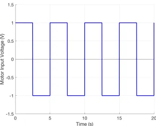
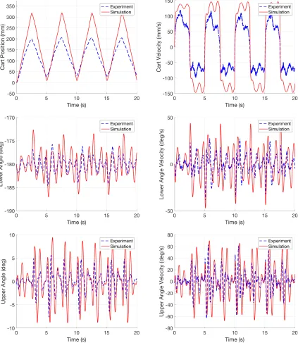
To validate our nonlinear model for the DIP system, we apply a set voltage input and compare the measured performance of the real system to the simulation results. The parameter values used for this simulation are given in Appendix A.2. Our input voltage is a square wave with an amplitude of 1 V and a frequency of 0.2 Hz as shown in Figure 2.3. Figure 2.4 shows the real-time experimental results in blue (dashed) and the simulation results in red (solid) with this voltage input. We can see that the simulation results generally follow the same patterns as the experimental results; however, the magnitude of the simulation results is typically larger than the experimental results. This is particularly apparent for the cart position. In order to address the discrepancies between the magnitudes of the model and the experimental results, we decided to use parameter estimation techniques on the friction values used in the model. In this way, we hope to improve our model accuracy relative to the experimental results.

We perform our parameter estimation on the three viscous damping coefficients as seen at the motor pinion,Bc, and the upper and lower pendulum axes,B1 and B2. The original values

for these parameters were given by Quanser for our system as

Bc= 5.4 N.m.s/rad, B1 = 0.0024 N.m.s/rad, B2 = 0.0024 N.m.s/rad.

Figure 2.3: Input voltage for use in model calibration.

squared errors between the model and the experimental results. We write this optimization problem as

q∗= arg min

q N

X

i=1

(yi−X(ti;q))T(yi−X(ti;q)) (2.46)

where q = [Bc, B1, B2] is the set of parameters to optimized. We let X be the state vector

solution to our nonlinear model with X = [xc(t), α(t), θ(t), x0c(t), α0(t), θ0(t)]. Then, N is the

number of experimental data points, and yi is the experimental data for a given time pointti.

Table 2.1: Optimized friction parameter values found using fminsearch.

Bc B1 B2 Bc∗ B1∗ B2∗ J

5.4 0.0024 0.0024 11.1878 0.03473 0.006230 4.391e+03 4.3 0.02 0.02 11.1747 0.03475 0.006224 4.391e+03 13 0.02 0.02 11.1925 0.03472 0.006228 4.391e+03 13 0.08 0.02 11.1951 0.03475 0.006224 4.391e+03 13 0.08 0.08 11.1997 0.03476 0.006211 4.391e+03

Figure 2.4. Using the optimized values in the first row of the table,

Bc= 11.1878 N.m.s/rad, B1 = 0.03473 N.m.s/rad, B2= 0.006230 N.m.s/rad,

we compare the new model values with the experimental values of each state. These results are shown in Figure 2.5. The values of the three position states from the model are much closer to the experimentally observed values. For the cart velocity, the overall magnitudes are much closer, though the model doesn’t capture the smaller changes in velocity on the 2.5 second sub-intervals as closely as the previous model did. The two states for the angular velocities of the upper and lower pendulums are generally closer to the experimental results, but now the values of the experimental results are actually slightly larger than those of the model.

Chapter 3

Stabilization Control of an Inverted

Double Pendulum System

In this chapter, we will discuss the stabilization of the double inverted pendulum system. We begin by discussing control methods currently used in the literature. Then we will derive a linear quadratic regulator controller and a power series based controller for the system. Both simulation and real-time experimental results will be presented for each controller.

3.1

Overview of Existing Control Methods

Control problems for the double inverted pendulum come in two varieties: swing-up and stabi-lization control. Swing-up control refers to beginning the pendulum at rest in its stable, down-ward hanging equilibrium state and then using a motor to bring the pendulum to its vertical, unstable equilibrium state and balancing it there. Stabilization control refers to just this second step, where the pendulum begins in the unstable equilibrium position and must be balanced there. Several control design approaches have been developed and applied to the DIP system for each of these cases. However, these methods are typically applied only in simulations and not on real-time experimental set ups. These simulations also frequently use simplified versions of the DIP model which ignore frictional effects.

We also note that the models seen in the literature are typically simpler than the one derived in Chapter 2 since the upper pendulum angle,θ, is measured from vertical rather than relative to the lower angle as we have done [7, 9, 13, 15, 18, 33, 43]. This reference point results in simpler model formulations but is not as easily applied to our real system since we can only measure θrelative to α.

that is frequently used as a baseline for comparison with other methodologies [7, 9, 40]. How-ever, since the DIP system is highly nonlinear and the LQR controller can only be applied to linear systems, this method requires that we first linearize about the unstable equilibrium

X= 0. Therefore, this method can only be used near the equilibrium as a locally near-optimal stabilizing control as shown in [7]. This control is also commonly used to perform the stabi-lization after using a swing-up control once the pendulum is within a certain basin near the equilibrium [43].

State Dependent Riccati Equation (SDRE) Control is a method which uses a non-linear form of the DIP model to develop a control that is dependent on the states. This method is sometimes considered to be a nonlinear extension of the LQR control. It has been shown to perform similarly to the LQR control when close to the equilibrium state and performs better at larger pendulum deflections [7]. However, this method can be very computationally expensive since it requires solving the state dependent Riccati equations at each time step.

Neural Networks allow for direct nonlinear optimization of a control. They are popular for controlling nonlinear systems because of their universal function approximation capabilities as discussed by Bogdanov in [7]. Due to the costs and challenges in training the neural networks, when used on their own, neural networks were unable to improve beyond the performance of the LQR control, only achieving stabilization in the same range. However, when combined with either the LQR or SDRE control, neural networks improved performance since they were able to generate “corrections” to the other controls, and in the case of the SDRE control, also achieved noticeable reductions in computational costs. Still, studies of this method have only been shown in simulation, often without limits on the magnitude of the control force.

Passivity Based Controlhas been used with partial feedback linearization, primarily for the swing-up of a DIP system as in [16, 43]. These are energy based methods where the stability is asymptotic to a manifold rather than a point, and therefore are typically used with LQR controls for stabilization. Again, only simulation results are typically presented, though [16] does include a detailed analysis of the motor performance in the construction of their control.

Feedforward/Feedback Controlsolves the swing-up control problem by solving an opti-mization problem where the unstable and stable equilibrium are boundary conditions and they seek to determine a path for the pendulum to follow for swing-up [13, 33]. These controllers then switch to a linear feedback control for the stabilization of the DIP. Experimental results have been presented in the literature for these controllers, but they are sensitive to the model parameters and therefore require optimizing the model parameters before applying them to the system [13].

Fuzzy Control methods attempt to stabilize the DIP system by constructing fuzzy rules that focus on each aspect of the system independently. They then use priority weighting to stabilize the complete system. This has been shown in simulation for a parallel double inverted pendulum, where two pendulums are mounted on a single cart but not connected to each other, but has not yet been applied to a DIP system of our type [41].

Sliding Mode Controlis a robust control method that uses a discontinuous control signal. However, it can lead to undesirable performance issues such as chatter when combined with fast switching times. This control has been used to stabilize the DIP system in [15] and numerical simulations are presented.

3.2

Problem Statement

Our goal is to stabilize the DIP system about its unstable, vertical equilibrium with minimal cart and pendulum movement and control effort. In particular, we desire the pendulum angles to never exceed a 10◦ deflection from the vertical position, that is,|α(t)|,|θ(t)| ≤10◦.To begin, we write the equations of motion for the DIP system in their state space representation as

X0(t) =f(X(t)) +Bu(t)

X(0) =X0

(3.1)

with state vector X(t) = [xc(t), α(t), θ(t), x0c(t), α0(t), θ0(t)]T and control variableu(t) =Vm(t).

We also consider the cost functional

J(X0, u) =

Z ∞

0

XTQX +Ru2dt (3.2)

where Q is a constant valued 6x6 symmetric and positive definite matrix, andR is a positive scalar.

Since we will be applying our controls to a real-time system, we have some additional constraints on our state variables. Our track length is finite, and therefore, for the safety of the system, we require that the cart does not run to the edge of the track. We assume the center of the track is at xc(t) = 0, so we require |xc(t)| ≤400 mm. We also need to ensure that the

power amplifier is not put into saturation by our applied control voltage, so we need to satisfy

3.3

LQR Control

First, we apply a standard linear quadratic regulator (LQR) controller to our system. Since this control is for linear systems, we must linearize the system about the zero equilibrium state. In practice, we accomplish this by using the Taylor function in Maple. Then we can write our system from (3.1) as

X0(t) =AX(t) +Bu(t)

X(0) =X0.

(3.3)

To determine the optimal control relative to the cost given in (3.2), we begin by considering the Hamiltonian function of this system given by

H(X, u, λ) = 1 2(X

T_QX+uT_{Ru) +λ}T_{(AX+Bu) (3.4)}

whereλis a Lagrange multiplier referred to as the costate. We follow the derivation of [20] which uses the calculus of variations to show that the necessary conditions to obtain a minimum cost for this problem are

Hx =−λ0 =QX +ATλ, (3.5)

Hλ =x0 =AX+Bu. (3.6)

For the unconstrained control problem, we would also have the stationarity condition given by

Hu= 0 =Ru+BTλ. (3.7)

Since in our problem, the input control is bounded, that is,|u(t)| ≤umax, we use Pontryagin’s

minimum principle which requires that

H(x∗, u∗, λ∗, t)≤H(x∗, u, λ∗, t) (3.8)

for all u in the admissible space with∗ denoting the optimal quantities. Using (3.4), we have

1 2(u

∗

)TRu∗+ (λ∗)TBu∗ ≤ 1

2u

T_Ru+λT_{Bu (3.9)}

for all admissible u. Therefore, we want to select our input to minimize the quantity 1₂uT_Ru+

λTBu. We add the term 1₂λTBR−1BTλsince it doesn’t depend on uand alternately minimize

1

Since R >0, we know this is equivalent to minimizing

1 2(u+R

−1_BT_λ)T_(u+R−1_BT_{λ). (3.11)}

If the magnitude ofR−1BTλ(t) is smaller thanumax, thenu∗ is found by setting the derivative

of (3.11) with respect tou equal to zero, that is,

u+R−1BTλ= 0. (3.12)

Thus,

u=−R−1BTλ (3.13)

if|R−1BTλ(t)| ≤umax. Note that this is the same result obtained using the stationarity

condi-tion given in (3.7). However, if|R−1BTλ(t)| ≥umax, then the result of minimizinguusing (3.12)

is an inadmissible value foru. Therefore, the best we can do is selectuto makeu+R−1BTλ(t) as close to zero as possible. Thus,

u=







umax ifR−1BTλ(t)<−umax,

−umax ifR−1BTλ(t)> umax.

(3.14)

Combining (3.13) and (3.14), we find that the optimal control for the constrained input is

u=



   

   

umax ifR−1BTλ(t)<−umax,

−R−1BTλ if|R−1BTλ(t)| ≤umax,

−umax ifR−1BTλ(t)> umax.

(3.15)

Note, that if|R−1BTλ(t)| ≤umax for allt, then this is the same control as in the unconstrained

control problem.

We now assume we are in the case where|R−1BTλ(t)| ≤umax and suppose that the costate

λis given by

λ=P X (3.16)

for some matrixP. Substituting (3.16) into (3.5) and (3.15) for this case, we obtain

−λ0 =QX+ATP X, (3.17)

We then substitute (3.18) into (3.6) to find

x0 =AX−BR−1BTP X. (3.19)

Then we differentiate (3.16) to obtain

λ0 =P X0 (3.20)

=P(AX−BR−1BTP X) =P AX−P BR−1BTP X.

Setting this equal to (3.17), we get

−QX−ATP X =P AX−P BR−1BTP X. (3.21)

This implies

P AX−P BR−1BTP X+QX+ATP X = 0 (3.22) (P AX+ATP−P BR−1BTP +Q)X = 0. (3.23)

Since this is true for allX, we have

P A+ATP−P BR−1BTP+Q= 0 (3.24)

which is the well known matrix Riccati equation. Thus, the feedback control is given by

u=



   

   

umax ifR−1BTP X <−umax,

−R−1BTP X if|R−1BTP X| ≤umax,

−umax ifR−1BTP X > umax.

(3.25)

whereP is the solution to the matrix Riccati equation given by (3.24).

3.3.1 An Application Example

As an exercise, we consider the following nonlinear system

x00(t) + sin(x(t)) =u(t). (3.26)

representation as

X(t)0=f(X(t)) +Bu(t) (3.27)

where

f(X(t)) =



 

x2

−sin(x1)

  , B =    0 1   .

In order to apply the LQR control, we begin by linearizing our system about the solution

X= [0,0]T. Then our linearized system is

X0(t) =AX(t) +Bu (3.28)

where A=    0 1

−1 0

  , B =    0 1   .

We consider the cost functional

J(X0, u) =

Z ∞

0

(XTQX +Ru2)dt (3.29)

where Q=    40 0 0 30   

R= 10.

P to the algebraic Riccati equation and the control gain,

K =R−1BTP. (3.30)

Figure 3.1 shows the trajectories of the states of the system for an initial state ofX(0) = [2,1]T and the control effort. We can see that the LQR controller quickly drives the states to zero as desired.

(a) (b)

Figure 3.1: LQR control applied to example problem: (a) state trajectories and (b) control effort.

3.4

Nonlinear Control

We now consider the nonlinear system as given in (3.1) with cost (3.2). It is shown by [10] that the optimal nonlinear feedback control is of the form

u∗(X) =−1

2R

−1_BT_V

X(X) (3.31)

where the functionV is the solution to the Hamilton-Jacobi-Bellman (HJB) equation given by

V_XT(X)f(X)−1

4V

T

X(X)BR −1_BT_V

3.4.1 Power Series Based Controller

Since the HJB equation is difficult to solve analytically, the main challenge to using the optimal control given in (3.31) is how to determine V(X). Various efforts have been made to use a numerical approximation of the HJB equation to obtain a suboptimal control. We will follow Garrard and others [10, 11, 12] to numerically approximate the solution of the HJB equation from (3.32) using its power series representation:

V(X) =

∞

X

n=0

Vn(X), whereVn(X) =O(Xn+2). (3.33)

We also rewrite the nonlinear function f from (3.1) as

f(X) =A0X+

∞

X

n=2

fn(X), where fn(X) =O(Xn). (3.34)

We then substitute these expansions into the HJB equation to obtain

∞

X

n=0

(Vn)TX

!

A0X+

∞

X

n=2 fn(X)

! −1 4 ∞ X n=0

(Vn)TX

!

BR−1BT

∞

X

n=0

(Vn)X

!

+XTQX = 0.

(3.35)

Next, we separate out the terms according to powers of X to get a series of equations:

(V0)TXA0X−

1 4(V0)

T XBR

−1_BT_(V

0)X +XTQX = 0, (3.36)

(V1)TXA0X+ (V0)TXf2(X)−

1 4(V1)

T

XBR−1BT(V0)X −

1 4(V0)

T

XBR−1BT(V1)X = 0, (3.37)

(Vn)TXA0X+

n−1

X

k=0

((Vk)TXfn+1−k(X))−

1 4

n

X

k=0

((Vk)TXBR−1BT(Vn−k)X) = 0, (3.38)

wheren= 2,3,4, . . .

Equation (3.36) can be solved by

V0(X) =XTP X (3.39)

whereP is the solution to the matrix Riccati equation (3.24). To solve (3.37), substitute in the equation

to obtain

(V1)T_XA0X+ 2XTP f2(X)−1

2(V1)

T XBR

−1_BT_{P X−}1

2X

T_{P BR}−1_BT_(V1)

X = 0. (3.41)

We rearrange terms to find

XT AT₀(V1)X + 2P f2(X)−P BR−1BT(V1)X

= 0. (3.42)

Since this is true for allX, we can then solve for (V1)X to obtain

(V1)X =−2(AT0 −P BR−1BT)−1P f2(X). (3.43)

We take the sum of (3.40) and (3.43) as an approximation for VX. Then, substituting into

(3.31), we obtain a quadratic feedback control law:

u∗(X) =−R−1BT

h

P X− AT₀ −P BR−1BT−1P f2(X)

i

. (3.44)

In our DIP modelf2(X) = 0, so we consider (3.38) withn= 2, and our control is

u∗(X) =−R−1BT hP X− AT₀ −P BR−1BT−1

P f3(X)

i

. (3.45)

3.4.2 An Application Example

As an exercise, we again consider the example system from Section 3.3.1. To apply the power series based controller, we first take the necessary derivatives of f to find the power series representation

f(X(t)) =



 

x2

−sin(x1)





, (3.46)

=



 

x2

−x1+ 1₆x3₁+O(x5₁)





. (3.47)

From this we can see that the termf2(X) = 0, so we use the control

u∗(X) =−R−1BT hP X− AT₀ −P BR−1BT−1

P f3(X)

i

. (3.48)

that in comparison to the LQR controller, when using the power series based control, the states reach zero slightly faster.

(a) (b)

Figure 3.2: Power series based control applied to example problem: (a) state trajectories and (b) control effort.

3.5

Simulation Results

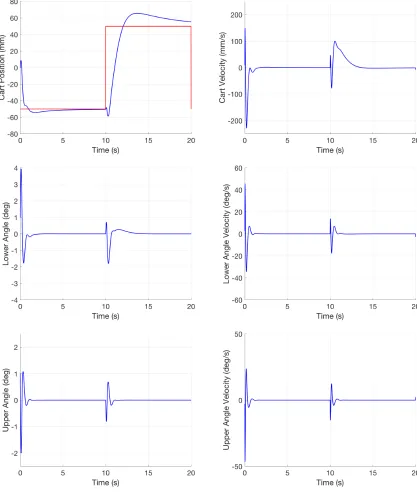
Prior to implementing either stabilization controller on the real-time DIP system, we check the performance in simulation using MATLAB Simulink. The initial condition for the simulations is to have the cart at rest at a position of 0 mm and both the upper and lower pendulum angles are deflected to 1 degree, i.e.X= [0, 1, 1, 0, 0, 0]T. We require the cart’s position to track a square wave with amplitude 50 mm and a frequency of 0.05 Hz.

Figure 3.3: Simulation results for the state trajectories using the LQR controller with

Figure 3.4: Control effort for the simulation using the LQR controller with

Q= diag(30,350,100,0,0,0) andR= 0.1.

3.6

Experimental Results

3.6.1 Experimental Apparatus

As previously stated, our experimental apparatus for the DIP system was provided by Quanser Consulting, Inc. as shown in Figure 1.2 and described in Section 1.1. The two pendulum rods are mounted on an IP02 linear servo unit; voltage is applied to the cart via a VoltPAQ amplifier; and communication between the computer and the system is provided by two Q2-USB DAQ control boards. Figure 3.5 shows a diagrammatic representation of the experiment. Detailed technical specifications are found in [31]. The real-time experiments are run using a desktop computer running Windows 7 with a 3.20 GHz Intel Core i5 650 processor and 4 GB of RAM.

3.6.2 Experimental Procedure

IP02 (Cart) Amplifier

DAQ Computer

Cart and Pendulum Encoders

Motor Connector

Amplifier Command

Control Signal

Pendulum Angles and Cart Position

Figure 3.5: A diagram of the experimental setup for the DIP system.

different controls for each experiment. Real-time experiments are begun with the pendulum in the downward, stable configuration, completely at rest. The position of the system at that time is considered to be atxc(0) = 0, α(0) =−180◦,θ(0) = 0◦. Once the real-time software is

running, we manually move the pendulum to the desired vertical, unstable equilibrium position. When the pendulum is within 0.5 degrees of the desiredα andθposition, that is, zero degrees, the feedback control turns on and will work to stabilize the pendulum.

Figure 3.6: Simulink block diagram governing the real-time implementation of the DIP system.

We implement each controller for a variety of Qand R values to assess the performance of the controller. In order to improve our controller’s performance, we adjust the values ofQ and

R according to the following guidelines:

2. If the pendulum does not meet the specifications for the angle, increaseQ22orQ33and/or

decrease Q11.

3. If the control voltage is too large or the cart vibrates excessively, increase R and/or decrease Q11,Q22, orQ33.

3.6.3 Results for the LQR Controller

To implement the LQR controller, we compute the solution to the matrix Riccati equation given in (3.24) using the lqr command in MATLAB. We then use the Simulink diagram shown in Figure 3.6 to apply the control to the real time system.

Figure 3.7 shows sample experimental results using the LQR controller with weighting matricesQ= diag(30,350,100,0,0,0) andR= 0.1. When performing the experiment, we allow the system to run for some time between one and three minutes to ensure that the pendulum system will remain stabilized, and here we show the behavior on a typical 20 second subinterval. The behavior seen here repeats over the course of the entire experiment. We can see that the position of the cart remains within 100 mm of the center of the track. The lower pendulum angle stays within 8 degrees of its vertical position, and the upper pendulum angle remains within 4.5 degrees of alignment with the lower rod. Examining the input voltage used to control the system shown in Figure 3.8, we see that, for this sample of the real-time experiment, the motor voltage remains less than 9 V. While the voltage is staying within its saturation limits, we would prefer the system to stay closer to the center of the track and the pendulums to be closer to vertical. Keeping this in mind, we can then adjust the weighting matrices Qand R in pursuit of better system performance.

We adjusted theQ andR values used in the LQR controller and summarize the results for the state trajectories and the motor input voltage as shown in Table 3.1. We see that for some tested controllers, the amplifier enters voltage saturation at least once resulting in a maximum applied voltage of 10 V. However, we note that just because the maximum voltage was not at the saturation level, this does not always correspond to a lower average or cumulative motor voltage. For example, compare the second and third lines of the table. In the third tested case the amplifier enters saturation at least once, but the average and cumulative motor voltages are less than the second tested case where the amplifier did not enter saturation.

Figure 3.7: Real-time experimental results for the state trajectories using the LQR controller with

Figure 3.8: Control effort for the real-time experiment using the LQR controller with

Q= diag(30,350,100,0,0,0) andR= 0.1.

We also attempt to keep the cart closer to the center of the track by increasing the value of the weight on the cart position,Q11. The resulting control is shown in the third line of Table 3.1, and the average and maximum values for the cart position are smaller than previously seen, though not by a significant amount. The average angular positions are slightly larger than with the original control, but the control effort is similar on average.

The next tested case explored weighting the velocity states to see the effect on the system performance. When larger weights were applied to the velocity states, the pendulum failed to stabilize, so we restricted ourselves to small ones. With this control, the average and maximum values for the states and the voltages increased slightly in comparison to the previously tested values. However, this control was more likely to fail to stabilize the pendulum in general.

Table 3.1: Maximum and average values for the states and control voltages using the LQR controller with various values ofQandR. (xc[mm],α[degrees],θ[degrees],Vm[V]).

max|xc| max|α| max|θ| max|Vm|

Q R

avg|xc| avg|α| avg|θ| avg|Vm|

R20

0 |Vm|dt

94.5884 7.5586 4.2188 8.5906 diag(30,350,100,0,0,0) 0.1

29.4310 3.4183 1.8656 1.6646

33.2370

86.3535 7.9102 4.4824 5.8618 diag(30,350,100,0,0,0) 0.5

34.1592 4.5009 2.3253 2.1029

41.6019

92.0634 8.7891 5.0098 10

diag(100,300,100,0,0,0) 0.1

28.8757 4.1876 2.4168 1.9954

39.7388

79.3924 7.9980 4.1309 10

diag(100,300,100,1,1,1) 0.1

31.4460 3.8657 1.9683 2.1865

43.5259

133.3975 15.9961 8.6133 10 diag(200,300,100,0,0,0) 0.5

64.2152 9.6711 5.4195 4.1135

81.4041

112.4916 14.1504 6.7676 8.7765 diag(100,300,100,0,0,0) 1.0

58.9119 8.1359 4.1689 3.3851

67.4756

the pendulum.

Lastly, we tried just increasing the weight on the control voltage toR= 1.This resulted in poorer performance of the state variables, and this was also a control which was more likely to fail to stabilize the pendulum at all.

3.6.4 Results for the Power Series Controller

We implement this power series based control for the same values ofQandRas were used with the LQR controller. Figure 3.9 shows the sample experimental results using the first control,

Q = diag(30,350,100,0,0,0) and R = 0.1, and Figure 3.10 shows the control effort. Again, we run each experiment for between one and three minutes, and we show the behavior on a typical 20 second subinterval. The behavior shown continues throughout the experiment. While the control voltage Vm does reach a saturation level of 10 V a few times, it is mostly during

Figure 3.10: Control effort for the real-time experiment using the power series based controller with

Q= diag(30,350,100,0,0,0) andR= 0.1.

looking at the plot of the cart position, we can see that the system had a short period of more jagged motion which is typically seen when the pendulum is very close to the zero state, as confirmed by the plots of the upper and lower pendulum angles. This behavior occurs regularly with the power series based controllers, but never continues for longer than five seconds before returning to the patterns shown in the rest of the figure. Otherwise, the motion is quite similar to that for the LQR controller with the same weighting matrices. The cart position remains within 100 mm of the center of the track, and the lower and upper angles remain within 6 and 5 degrees of their zero states, respectively. In fact, while the average position of the cart is farther from the center of the track than that obtained by the corresponding LQR controller, the average values for the upper and lower pendulum angles are significantly smaller. As seen in the first line of Table 3.2, the average angular states using the power series based controller are half the magnitude of the those using the corresponding LQR controller. Even so, this power series controller has average and cumulative motor input voltages only slightly higher than that applied by the LQR controller.

weighting matrices were also likely to cause the power amplifier to go into voltage saturation at some point, but, in general, average and cumulative applied motor voltages were lower than those seen with the LQR controllers.

Table 3.2: Maximum and average values for the states and control voltages using the power series based controller with various values ofQandR. (xc[mm], α[degrees],θ[degrees],Vm[V]).

max|xc| max|α| max|θ| max|Vm|

Q R

avg|xc| avg|α| avg|θ| avg|Vm|

R20

0 |Vm|dt

93.0870 5.2734 4.1309 10

diag(30,350,100,0,0,0) 0.1

36.4901 1.7754 0.9047 1.7517

34.7876

98.6832 7.6465 3.7793 6.6544 diag(30,350,100,0,0,0) 0.5

35.4940 3.1983 1.4241 1.6180

32.1967

72.0446 6.5918 4.5703 10

diag(100,300,100,0,0,0) 0.1

26.3484 2.8903 1.4913 1.8682

37.2777

62.4220 4.9219 3.2520 10

diag(100,300,100,1,1,1) 0.1

22.3453 2.0616 1.0954 1.7821

35.3103

113.5835 8.7891 5.0098 6.3668 diag(200,300,100,0,0,0) 0.5

39.8354 4.4707 2.0734 1.9491

38.7577

93.5648 7.8223 4.9219 10

diag(100,300,100,0,0,0) 1.0

40.0830 4.1154 1.7709 2.2386

44.6471

For the second test case where the weightRon the motor voltage was increased, we see that the applied voltage was less than that of case one, with R = 0.1, with the power series based controller. As expected, the values of the states were also higher on average, and thus further from the desired state. However, the state trajectory response was better than the corresponding LQR control for each of the pendulum angles and similar for the cart position.

makes sense since this control also has a slightly smallerQ22weight of 300. The applied voltage

for the control was close to the first case control which had the same value for R. Compared to the corresponding LQR controller, the state trajectories and applied motor voltage were smaller by all measures, showing better performance.

The fourth test case included nonzero weights for the velocity states. Again, including these weights resulted in controllers which did not always consistently stabilize the pendulum, so the value of the weights was kept low in comparison to those used for the position states. With the power series based controller, when stabilization was attained, the resulting performance was better than with many of the other tested controllers as shown in the table. This controller obtained the best results for the cart position, and was second only to the first test case for the performance of the pendulum rods and decreasing the control effort. This was also much better than the corresponding LQR controller. However, this was definitely the control that was most likely to fail to stabilize the pendulum at all.

For the fifth test case, we increased the weight on the cart position as well as the weight on the applied motor voltage. As was the case with the LQR control, the resulting power series based control had one of the worst overall performances in terms of both the state trajectories and the applied motor voltage, though it did perform better than the corresponding LQR control.

Lastly, we again tested the case with Q = diag(100,300,100,0,0,0) and R = 1.0 which places a high weight on the applied motor voltage. This case actually had the highest maximum, average, and cumulative applied motor voltage of the tested power series based controllers, as well as one of the worst performances for the state trajectories, attaining similar results to the fifth test case. The control did perform significantly better than the corresponding LQR controller. The average cart position was almost 20 mm closer to the center of the track; the lower pendulum angular position was 4 degrees closer to vertical, half the distance of the LQR controller; and the upper pendulum was over 2 degrees closer to its zero state, also half the distance of the LQR controller.

Chapter 4

State Observation for an Inverted

Double Pendulum System

To this point, we have tacitly assumed that we have access to all of the state variables in our model in order to compute our desired feedback controls. However, in both this and many other applications we do not actually have the ability to measure every state variable. Therefore, in order to compute our feedback controls we must first construct or estimate the unmeasured state variables. This is known as the state estimator or state observer problem which is shown diagrammatically in Figure 4.1. The partial measurements of the system model are passed as inputs for a state estimator. This estimator outputs a full set of state variables, including the measured states and the constructed states, to use as input for the feedback control. The control is then used as an input for the system model.

System Model Nonlinear State Estimator

Optimizer Predicted Outputs (partial measurements)

Estimated States

Cost Function Control Constraints

Future Controls

For the DIP system, our physical apparatus takes direct measurements of the three position state variables, xc, α, and θ, using three encoders. The three velocity state variables, x0c, α0,

and θ0, are not measured directly, so they must be estimated. We will first discuss the current method implemented to estimate these variables and then we will examine two other proposed estimators for this system.

4.1

Low Pass Derivative Filter

A low pass filter is a filter that works to reduce noise from a signal by passing signals with a frequency lower than a certain cut-off frequency and attenuating, or reducing, the signal strength of higher frequency signals. Removing some signals in this way creates a smoother signal and improves the ability to see trends and increases the overall signal-to-noise ratio. The particular cut-off frequency used is a design decision for the filter. In a first order low pass filter, the signal amplitude is reduced by half each time the frequency doubles for frequencies above the cut-off. A second order filter attenuates high frequencies more quickly, reducing the signal amplitude to one-fourth its original value each time the frequency doubles.

The general equation for a second order low pass filter in the transfer function domain is given by

H(s) = ω

2

n

s2_{+ 2ζω}

ns+ω2n

(4.1)

where ωn is the cut-off frequency and ζ is the damping ratio [30]. A derivative filter is then a

combination of passing a signal through a low pass filter and taking a derivative, which in the transfer function domain is given by

H(s) = ω

2

ns

s2_{+ 2ζω}

ns+ωn2

. (4.2)

We note that it is important to use a filter when taking a derivative of a signal since differen-tiating a signal amplifies the noise present in that signal.

As part of the Quanser provided software Quarc which communicates with the DIP system, a second order derivative filter is used when reading the data from the encoders to compute the velocity states. For the IP02 linear servo unit, the given values for design of the second order low pass filter are

ωcf1= 100π, ζ1= 0.9, ωcf2 = 20π, ζ2 = 0.9,

whereωcf1 is the cut-off frequency andζ1 is the damping ratio for the encoder which measures

the cart position andωcf2 is the cut-off frequency andζ2 is the damping ratio for the encoders

obtain the velocity states for the real-time experiments for use in our feedback controls as previously discussed in Chapter 3. However, we also explored other options to estimate these states.

4.2

Kalman Observer

The first observer we explored for the DIP system is the Kalman filter. This filter is constructed using linear systems, so we begin by considering a general linear system:

x0(t) =Ax(t) +Bu(t)

x(0) =x0.

(4.3)

We also need to consider our output equation, that is, an equation returning what is being observed,

y(t) =Cx(t) (4.4)

wherey∈_Rp _{andpis the number of observed states. In general, we can design a state observer}

ˆ

x so that it has the same dynamics as the original system which is given by

ˆ

x0(t) =Axˆ(t) +Bu(t) +G(y(t)−yˆ(t)) (4.5)

where

ˆ

y(t) =Cxˆ(t). (4.6)

The term G(y(t)−yˆ(t)) is the correction term. The observer gain G is designed to drive the state observer ˆxto the actual statex. To ensure that this happens, we define the error between the state observer and the actual state as

e(t) = ˆx(t)−x(t). (4.7)

We differentiate this equation and use the state equation (4.3) and the observer equation (4.5) to obtain

e0(t) = ˆx0(t)−x0(t)

=Axˆ(t) +Bu(t) +G(y(t)−yˆ(t))−Ax(t)−Bu(t) =A(ˆx(t)−x(t)) +G(Cx(t)−Cxˆ(t))

If all of the eigenvalues of (A−GC) have negative real parts, then the error e will approach zero, that is, the state observer ˆxwill approach the actual statex. This is true even if there are large errors between the initial observer and the actual state. This is known as the Luenberger observer [4].

In the state feedback problem, we use the state observer for feedback, so

u(t) =Kxˆ(t). (4.9)

We substitute this into the state equation (4.3) to obtain

x0(t) =Ax(t) +BKxˆ(t)

=Ax(t) +BK(e(t) +x(t)) = (A+BK)x(t) +BKe(t).

When we combine this with the error equation (4.8), we obtain the closed-loop system



 

x0(t)

e0(t)

  =   

A+BK BK

0 A−GC

     

x(t)

e(t)





 (4.10)

y(t) =

C 0   

x(t)

e(t)





. (4.11)

We note that the system matrix for the closed-loop system is a block triangular matrix, and therefore the eigenvalues of the system are the eigenvalues ofA+BK and A−GC. Thus, the design of the state feedback and the state observer can be done independently. This is known as the separation principle [4].

We will now show that the state observer described above is the Kalman filter when white noise processes are added to the state and output equations following the presentation in [14]. We begin by examining the linear filtering problem given by

x0(t) =Ax(t) +Bu(t) +g(t)w(t) (4.12)

yk =Cx(tk) +vk (4.13)

where measurements y are taken at discrete time points tk and w(t) and vk are uncorrelated