ABSTRACT
MA, YUE. A Multithreaded Real-time Robot for Embedded Design Space Exploration. (Under the direction of Dr. Alexander Dean.)
This thesis introduces an autonomous robot platform for real-time scheduling exper-imentation and benchmark suite to evaluate real-time optimizations and apply modern task scheduling methods.
It makes two contributions. First, it presents a reference hardware and software design for a line-following, obstacle-avoiding and maze-solving robot. This robot is based on a small commercially-available product. The software is structured as a multithreaded real-time system for use in evaluating scheduling approaches for cost-sensitive and resource-constrained applications. Second, it provides a detailed design space exploration showing the costs (processor speed and memory) of different scheduling approaches (static vs. dynamic and non-preemptive vs. preemptive).
A Multithreaded Real-time Robot for Embedded Design Space Exploration
by Yue Ma
A thesis submitted to the Graduate Faculty of North Carolina State University
in partial fulfillment of the requirements for the Degree of
Master of Science
Computer Engineering
Raleigh, North Carolina 2010
APPROVED BY:
Dr. Edward Grant Dr. James Tuck
DEDICATION
BIOGRAPHY
ACKNOWLEDGEMENTS
First and foremost, I would like to offer my sincere thanks to my parents, who love me and always believe in me. No matter what happens, they always encourage and support me in my endeavors.
I would also like to express my deep gratitude to my advisor, Dr. Alexander Dean, not only for giving me the opportunity of this study, but also for his advice throughout the work and his encouragement. I could not have completed my thesis without his guidance.
My heartfelt appreciation goes to Dr. Edward Grant and Dr. James Tuck for taking valuable time out of their schedule to serve as members of my advisory committee.
I am also very thankful to Sang Yeol Kang for providing his toolchain of LPC-H2888 board and his static timing analysis tool named ARMSAT, both of which helped me save much time.
TABLE OF CONTENTS
List of Tables . . . vii
List of Figures . . . viii
Chapter 1 Introduction . . . 1
Chapter 2 Related Work . . . 3
Chapter 3 Design Description . . . 5
3.1 Hardware Description . . . 5
3.1.1 3pi Robot . . . 6
3.1.2 Odometers . . . 6
3.1.3 LPC-H2888 Board . . . 6
3.1.4 LCD . . . 7
3.1.5 Sonar Range Finder . . . 7
3.1.6 Hardware Summary . . . 7
3.2 Software Description . . . 9
3.2.1 Tasks on ATmega168 MCU . . . 9
3.2.2 Tasks on LPC2888 MCU (FreeRTOS) . . . 11
3.2.3 Software Summary . . . 16
Chapter 4 Experiments and Results . . . 17
4.1 Practical Approach . . . 18
4.1.1 Environment . . . 18
4.1.2 Method . . . 19
4.1.3 Results . . . 21
4.1.4 Summary . . . 23
4.2 Theoretical Approach . . . 23
4.2.1 Limitation of Analysis Tool . . . 23
4.2.2 Results . . . 24
4.3 Summary . . . 25
Chapter 5 Analysis and Conclusion . . . 26
5.1 Static Scheduling . . . 26
5.2 Dynamic Scheduling . . . 27
5.2.1 Non-preemptive Scheduling . . . 28
5.2.2 Preemptive Scheduling . . . 31
Chapter 6 Future Work . . . 35
References . . . 37
Appendix . . . 39
Appendix A Instructions to Build the Robot . . . 40
A.1 Hardware Parts . . . 40
LIST OF TABLES
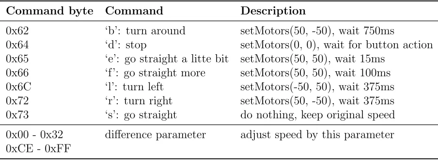
Table 3.1 Commands to control the robot . . . 9
Table 3.2 Two types of packet format . . . 12
Table 4.1 Period of each task . . . 20
Table 4.2 BCET and WCET using practical approach . . . 23
Table 4.3 Functions we need to measure . . . 24
Table 4.4 BCET and WCET using theoretical approach . . . 24
Table 4.5 Final BCET and WCET of each task . . . 25
Table 5.1 New WCET of each task for non-preemptive scheduling . . . 29
Table 5.2 WCET of each task for preemptive scheduling . . . 31
LIST OF FIGURES
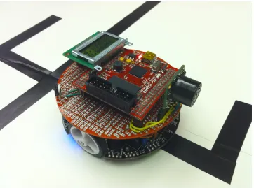
Figure 3.1 Robot we build in this project . . . 5
Figure 3.2 Wheel encoder disc . . . 6
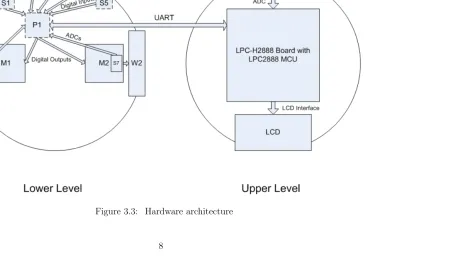
Figure 3.3 Hardware architecture . . . 8
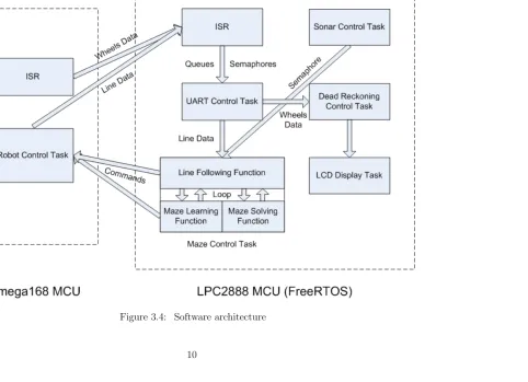
Figure 3.4 Software architecture . . . 10
Chapter 1
Introduction
Scheduling approaches overview
Normally, we can split different scheduling approaches into static approaches and dynamic approaches depending on whether we can schedule the tasks in different orders based on importance. A static approach schedules the tasks by specific and fixed order and we cannot change this order at any time, such as round robin scheduling. A dynamic approach schedules tasks based on importance (priority). Based on when the scheduler should schedule the next task to run, we have non-preemptive scheduling and preemptive scheduling approaches. In non-preemptive scheduling, the scheduler schedules the next task to run only when current task finishes. In preemptive scheduling, the scheduler schedules the next task to run when it needs to. Based on different methods that scheduler uses to decide how to schedule the next task, we have Rate Monotonic (RM) scheduling and Earliest Deadline First (EDF) scheduling approaches. In RM scheduling, tasks have fixed priorities which are decided by their periods. In EDF scheduling, tasks have dynamic priorities which are decided by whose deadline is the earliest from current time.
Our robot
In this thesis, we build an autonomous multithreaded real-time robot platform to explore embedded design space. We can use this robot to evaluate real-time optimization and apply different scheduling approaches to see the corresponding costs.
flash memory so it is difficult for us to do some relatively complicated computation like dead reckoning information calculation and it is also difficult for us to port a real-time operating system to achieve multithread in this microcontroller. Second, it has very lim-ited available pins, so we cannot add much hardware to the robot. But it still has many advantages such as built-in motors, wheels and five digital sensors which make the robot more autonomous and functional.
Connecting the 3pi robot to the LPC-H2888 board will bring us a small autonomous robot body and a multithreaded real-time robot heart. We can perform real-time schedul-ing experimentation on the robot. It is also very expandable so that we can add any hardware we need and implement the corresponding task to control the hardware since we run FreeRTOS (a real-time operating system) on the LPC2888 microcontroller.
The rest of the thesis is organized as follow:
Chapter 2 shows some related work of different scheduling approaches and some re-lated robots implementation.
Chapter 3 introduces the detailed hardware parts and software architecture design of the robot and their connections and relationship such as how they interact with each other.
Chapter 4 builds a test environment to get each task’s timing information using practical approach and theoretical approach.
Chapter 5 presents an analysis of schedulability based on different scheduling methods and explores the minimum microcontroller clock speed of the system under different scheduling approaches.
Chapter 2
Related Work
Schedulability analysis
Research on schedulability analysis of different scheduling approaches is wide and deep over the past 30 years for both static and dynamic priority scheduling approaches. [1] shows what the least upper bound to processor utilization is for a set of tasks with fixed priority order, if the tasks are schedulable. We can then use the least upper bound to test the schedulability under preemptive Rate Monotonic (RM) scheduling approach. It also shows that full processor utilization can be achieved by dynamically assigning the priories on the basis of their current deadlines which we can use to test the schedula-bility under preemptive Earliest Deadline First (EDF) scheduling approach. [2] shows a necessary and sufficient condition for schedulability under non-idling non-preemptive EDF scheduling approach. [3] shows that RM priority assignment is optimal for non-preemptive scheduling when each task’s relative deadline is equal to its period. We can use this result to test the schedulability under non-preemptive RM scheduling approach. [4] shows how to check the schedulability under static scheduling approach with helper interrupts.
Robot implementation
Chapter 3
Design Description
3.1
Hardware Description
Figure 3.1 shows the real photo of the robot we build in this project. We will focus on introducing the parts we add or the changes we make to the 3pi robot in this chapter.
3.1.1
3pi Robot
The 3pi robot is a small autonomous mobile robot designed by Pololu Corporation. It features two micro metal gear motors, five digital reflectance sensors, one 8×2 character LCD, one buzzer, and three user pushbuttons. It is based on an Atmel ATmega168 mi-crocontroller (8-bit AVR architecture) running at up to 20MHz with 16KB flash memory and 1KB SRAM. In this project, we mainly use the ATmega168 microcontroller, two gear motors and five digital reflectance sensors from the original 3pi robot.
3.1.2
Odometers
We add two odometers made of two analog reflectance sensors to the 3pi robot in order to monitor the black and white stripes which we stick on the two wheels (Figure 3.2). This allows us to get the wheel rotation information to calculate how much the robot moves which can be used for calculating the dead reckoning information. Details please refer to section Dead Reckoning Control Task.
Figure 3.2: Wheel encoder disc
3.1.3
LPC-H2888 Board
3.1.4
LCD
The LCD we use is a basic 8×2 character LCD which has a standard HD44780 parallel in-terface. It will display the dead reckoning position coordinates while the robot is running. This LCD is connected to LPC-H2888 board through the the LPC2888 microcontroller’s LCD interface.
3.1.5
Sonar Range Finder
The sonar range finder can detect objects from 0m to 6.45m (21.2ft) with a resolution of 2.5cm (1in) for distances beyond 15cm (6in). It runs on 3.3V provided by the LPC-H2888 board. The analog output is 6.45mV/inch ((Vcc/512)/inch) when the input voltage is 3.3V. We use it to detect obstacles while the robot is running so that the robot will do some actions to avoid the obstacles. Details please refer to section Sonar Control Task.
3.1.6
Hardware Summary
Figure 3.3 shows all the hardware parts in this project and how they interact with each other. The relationship and connections among the different parts are described as follows:
We make a maze using a black line on a white board so the ATmega168 microcontroller can monitor the five digital reflectance sensors to detect the line information, and then it will send the information back to the LPC2888 microcontroller through the UART connection. Then the LPC2888 microcontroller will send a movement command or a difference parameter (a parameter to adjust two wheels speed) back to tell the robot what the next movement is or the speed at which it should operate.
3.2
Software Description
Figure 3.4 shows all the tasks running on the ATmega168 microcontroller and LPC2888 microcontroller and their interactions. The task on the ATmega168 microcontroller side runs under static scheduling with an interrupt. The tasks on the LPC2888 microcontroller side run on FreeRTOS which provides multithreaded scheduling.
3.2.1
Tasks on ATmega168 MCU
In the following task and ISR, we use some basic interface functions from the 3pi robot library such as sending and receiving data through UART, setting motor speed and getting ADC value etc. to help us achieve the functions we need.
Robot Control Task
This task is running on the ATmega168 microcontroller. Its main function is getting the line information through the five digital reflectance sensors, sending them to the LPC2888 microcontroller and waiting for response commands to drive the robot. There are two types of commands: one type is movement command, such as “turn left”, “turn right” and “turn around” etc. The first part of Table 3.1 shows the movement commands to control the robot.
Table 3.1: Commands to control the robot
Command byte Command Description
0x62 ‘b’: turn around setMotors(50, -50), wait 750ms
0x64 ‘d’: stop setMotors(0, 0), wait for button action 0x65 ‘e’: go straight a litte bit setMotors(50, 50), wait 15ms
After decoding the commands, it will set a fixed speed to the two motors to achieve the corresponding movement. The other type of command is used for controlling the robot to follow the line. The value of each command is a number from -50 to 50 which is used to adjust the speeds of the two wheels. We use a simple PID control here, so the speeds of the two wheels are dynamic. The detail of this implementation is described in section Maze Control Task. The second part of Table 3.1 shows all the difference parameter commands to control the robot.
Below is how we set the wheel speed based on the difference parameter which the ATmega168 microcontroller receives:
i f( cmd < 0 )
s e t M o t o r s ( l e f t W h e e l S p e e d + cmd , r i g h t W h e e l S p e e d ) ;
e l s e
s e t M o t o r s ( l e f t W h e e l S p e e d , r i g h t W h e e l S p e e d − cmd ) ;
In this project, we set the values of the “leftWheelSpeed” and “rightWheelSpeed” at 50 (15cm/s). The maximum value is 255 which means the maximum speed of the robot is 1m/s.
Interrupt Service Routine
The ISR in the ATmega168 microcontroller side is triggered by a timer every 4ms. It will check the values of the two analog reflectance sensors and send them to the LPC2888 microcontroller. Since we only set the maximum speed of the wheels at 50 which is 15cm/s and about 15ms/stripe, 4ms frequency is fast enough to catch every stripe.
3.2.2
Tasks on LPC2888 MCU (FreeRTOS)
In this section, when we implement the functions for PID control and maze solving, we refer to the algorithm used in the original 3pi robot.
Interrupt Service Routine
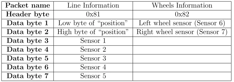
Based on section 3.2.1 Tasks on ATmega168 MCU we know there are two kinds of information that the LPC2888 microcontroller will receive. One is the line information, and the other is the wheels information. When the ATmega168 microcontroller side sends these two kinds of information, it will pack them in the corresponding format by adding headers, disassembling data and sending them in order. Because UART can only transmit one byte of data at one time, we need to disassemble the data whose value is larger than 255 by sending the low 8-bit data first and then the high 8-bit data of a 16-bit “int” type value. The two different types of format are described in Table 3.2.
Table 3.2: Two types of packet format
Packet name Line Information Wheels Information
Header byte 0x81 0x82
Data byte 1 Low byte of “position” Left wheel sensor (Sensor 6)
Data byte 2 High byte of “position” Right wheel sensor (Sensor 7)
Data byte 3 Sensor 1
Data byte 4 Sensor 2
Data byte 5 Sensor 3
Data byte 6 Sensor 4
Data byte 7 Sensor 5
Based on the five digital reflectance sensors, we calculate where the line is as the “position” variable. Its value is from 0 to 4000. 0 means the line is right under sensor 1 and 4000 means the line is right under sensor 5. If the line is out of the range of the sensors, its value may be 0 or 4000 which depends on from which side the robot goes off the line.
UART Control Task
Every time this task runs, it will check the line information and wheels information semaphores to see if they are ready in the receiving queue. If they are, it will extract the data bytes from the receiving queue in order, reassemble them and send them to the corresponding queues (line information queue and wheels information queue). If not, it will exit and reenter to check again based on the task’s period while the task is running. There are four reasons why we do not let this task suspend after finishing processing the data and resume it in the ISR when the data in receive queue is ready. First, in FreeRTOS or other real-time operating system, suspending or resuming a task may take longer time than the normal function we have in this task and during that time it will disable all the interrupts which may cause it to miss some input data or other unfore-seen errors. Second, we should make ISR execution time as short as possible. Third, although the way we implement the system means it needs to check line information and wheels information semaphores every time the task starts running, it takes less time than suspending and resuming tasks. Fourth, it meets the assumption “All tasks are independent” we use to analyze the schedulability in chapter 5.
Sonar Control Task
This task will get the sonar value through the 10-bit ADC which works in continuous conversion mode. Because the reading rate of the sonar range finder is 20Hz (50ms), we do not need to keep this task running all the time, therefore we can set a delay after every reading. We choose 40ms here which can allow enough time to read every sonar’s value, so the period of this task is about 40ms.
Dead Reckoning Control Task
This task mainly focuses on calculating the dead reckoning information. Every time it runs, it will check if there are some wheels data in the wheels information queue. If so, it will extract the data and calculate the coordinate of the robot based on the information. Here are two models that are used in different situations. One is only for line-following and obstacle-avoiding. In this model, the track can be any shape, such as round, rectangle or any other irregular shape. Because the resolution of the wheel stripe is limited, in order to calculate more accurate coordinates, we do not use PID control in this model which means we do not set the speed of the two wheels at the same time. We only set one wheel’s speed at one time and keep this wheel rotating some time, so we can require more accurate stripe information for calculation. But we may have less line tracking ability. In this model we display the coordinates and angle information on the LCD.
The other model we use is for maze-solving. The lines of a maze we build are all perpendicular, so we do not need the same stripe catching ability as the one in former model. Instead, we need more strong line tracking ability in order not to enter an intersection with an angle. If it enters an intersection with an angle, it cannot detect the intersection precisely using the five digital reflectance sensors we have in the robot, so we use PID control here which will be described in the next section to enhance line tracking ability. At this point, it is difficult to calculate the angle information based on the resolution we have in the wheel stripe if the line is not straight, so we only display the coordinates on LCD. Since all the lines are perpendicular, there is indeed no need to calculate the angle or direction.
Maze Control Task
This is a core task in this project. It mainly includes three functions: line following, maze learning and maze solving. We will describe them separately.
it goes back to the line. If the obstacle semaphore is not set, it will use a simple PID control method to calculate the speed difference parameter in order to control the robot to follow the line. We use the following equations to get the difference parameter:
dif f erence=proportional/60 +integral/30000 +derivative/2
This “difference parameter” is one type of the commands we discuss in section 3.2.1 Tasks on ATmega168 MCU. It should be between -50 and 50 because the robot’s maxi-mum speed is set to 50. The other variables we calculate as follows:
proportional=position−2000 integral=Xproportional
derivative=proportional−lastP roportional
The parameters for adjusting such as “60”, “30000”, and “2” are all based on exper-iment and observation. The value of “proportional” has the largest effect to the final difference value. For example, if we reduce the parameter “60” to “10”, the reaction of the robot to the line will be very big so that the robot will turn sharply to go back the line if it is off the line. If we increase the parameter “60” to “100”, the reaction of the robot to the line will be very small which means it will take more time to go back to the line if the robot goes off the line.
After getting the difference parameter, this function will send it to the ATmega168 microcontroller and then go back to the very beginning to run the loop again.
This function also analyzes the values of five digital reflectance sensors. If an in-tersection is found, it will return and go to the maze learning function to do further analysis.
direction for simplifying the path which is used for solving the maze and determining angle or direction which is used for the dead reckoning task to calculate the coordinates. Every time the robot finishes turning, this function will simplify the paths, so the record always keeps the shortest path from starting point to current location.
Maze Solving Function This function is relatively simple. When the robot redoes the maze and faces an intersection, it will jump to this function. It will help decide which turn the robot should take based on the simplified path record, so when the robot redoes the maze, it will follow the shortest path.
LCD Display Task
Since in this project we only have the coordinates information to be displayed on the LCD, we do not need use semaphores. When this task finishes running, it will be delayed for about 250ms. To achieve this we add a 250ms delay at the end of this task, so the coordinates information will be displayed about every half second which is the period of this task.
3.2.3
Software Summary
Chapter 4
Experiments and Results
In this chapter we use two traditional approaches to estimate each task’s execution time including BCET (Best Case Execution Time) and WCET (Worst Case Execution Time) in our robot platform. Especially after getting the WCET bounds, we can apply differ-ent scheduling policies to the system based on schedulability. We can also reduce the microcontroller’s clock speed to minimum under different scheduling policies because we know the WCET bound and each task’s period in certain clock speed.
WCET. But the estimation is still referable since we analyze most of the codes using the theoretical method. If the WCET we get from theoretical approach is larger than that from practical approach, we can use it as the final WCET for analysis. We will present more details in section 4.2 Theoretical Approach.
4.1
Practical Approach
4.1.1
Environment
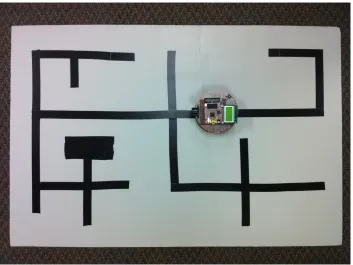
Figure 4.1 shows a simple maze we build for the robot to test and estimate timing information. Although it is simple, it includes all the possible intersections such as four-way, left turn three-four-way, right turn three-four-way, left turn two-four-way, right turn two-way and dead end etc. The black area made by three short tapes is the ending point. If we use the lower right entrance as the starting point, the robot will go through the whole maze since we use the “right hand rule” here.
4.1.2
Method
Task Period
To decide the microcontroller utilization and to get the minimum clock speed for the program based on different scheduling policies, we need to know each task’s period. We can also assume the period is also the task’s deadline in order to meet the assumptions for analysis in chapter 5. Here is how we get the periods. We set a counter to each of the five tasks and let the robot follow the line. Then we use a stopwatch to get the total time and from the counter we can get the total counts for each task, so now we know what the period of each task is by dividing the total time by the total counts.
After getting these real average periods, for analysis convenience and safety, we will fix these periods by some proper larger values. That is although these tasks run at larger periods, they still work well. For the sonar control task, the sonar range finder’s read rate is only 20Hz that is 50ms. In order to save the microcontroller utilization and also get the sonar reading result on time, we can set the delay time to 40ms, so the period should be about 40ms. The LCD display task is almost the same. We add a 250ms delay at the end of the task, so the period is about 250ms. We choose 250ms because we need to consider both user experience and task utilization which means this period should not be too big or too small. For the maze control task, we fix the period to 5ms for safety and convenient analysis reasons. Also because of the wheels data arriving every 4ms, we fix the period of the dead reckoning control task at 4ms although it may not run so frequently. For the UART control task, since it checks both line data semaphore and wheels data semaphore every time it runs, we just need to set the period at a certain value which is less than the minimum value between the period of the maze control task and the period of the dead reckoning control task, so we fix the period at 3ms in order to get the line data and wheels data from the ISR on time.
When we use non-preemptive scheduling policies, we need to add the ISR period to each task’s WECT because the tasks can be preempted by the ISR, so we separate the ISR from other tasks in the table. Its period equals 10bits / 115.2kbit/s = 86.7us. 115.2kbit/s is the UART speed. 10bits equals 1 date byte + 1 start bit + 1 stop bit. Table 4.1 shows the period of each task.
Table 4.1: Period of each task
Task Name Period
UART Control Task 3ms Sonar Control Task 40ms Dead Reckoning Control Task 4ms Maze Control Task 5ms LCD Display Task 250ms
ISR 86.7us
Task Execution Time
For estimating, we run the robot to solve the maze and measure the clock ticks for each task using a timer. To help analysis, we do not only measure the five tasks’ execution time, but also some important functions including the ISR in the program. We run the LPC2888 microcontroller at 60MHz and ATmega168 microcontroller at 20MHz. We use the following piece of code to count the clock ticks of the task or the function execution time we want to estimate:
t i m e r S e t C o u n t ( 1 , 6 0 0 0 0 0 0 0 0 ) ; // R e s t a r t t i m e r
// Put t a s k o r f u n c t i o n t o b e measured h e r e .
counterNew = 6 0 0 0 0 0 0 0 0 − timerGetCount ( 1 ) ;
i f( counterMax == 0 ) {
counterMax = counterNew ;
coun terMin = counterNew ;
} e l s e {
i f( counterNew < count erMin )
coun terMin = counterNew ; // Get new minimum t i c k
e l s e i f( counterNew > counterMax )
counterMax = counterNew ; // Get new maximum t i c k
Since our LPC2888 microcontroller’s clock speed is 60MHz, setting the counter to 600000000 means the timer can count up to 10 seconds. This is just for safety reasons, and normally the timer will not count down to 0 because we do not have such long tasks or functions even if they may be preempted. While solving the maze, each task or function will run many times, so we always monitor to update the maximum and minimum ticks. After solving the maze, we know the BCET and WCET of this round. We measure three times for each task or function in order to get more accurate results.
Since our robot system is highly based on the input and output like the data trans-mission between the ATmega168 microcontroller and the LPC2888 microcontroller, we cannot simply simulate it in some debuggers. We have to test it in the real environment in order to get results.
4.1.3
Results
Since each task or function has different situation, we discuss them separately below:
UART Control Task
The BCET of this task should happen when both of line information semaphore and wheels information semaphore are not set, so the task will go back again when it runs next time. The WCET should happen when both of line information semaphore and wheels information semaphore are set and both spend the maximum time to receive all the data bytes. Our test shows the BCET of this task is 200 ticks and the WCET is 17065 ticks.
Sonar Control Task
Dead Reckoning Control Task
For this task the BCET should happen when there is no wheels data in the wheels information queue. The WCET should happen when it calculates the coordinate with the most complicated data computation. Our test shows the BCET is 594 ticks and the WCET is 3460 ticks.
Maze Control Task
When the robot enters an intersection, the ATmega168 microcontroller needs to perform turning, so there is no input from the ATmega168 microcontroller which causes the UART control task and dead reckoning control task not work during that time. When we say BCET or WCET of this task, we mean the line following function which runs like a task when the robot follows the mazes, so the scheduler actually schedules the line following function. Our test shows the BCET of this function is 655 ticks and the WCET is 4476 ticks. We also record some other functions in this task to help us analyze. The BCET of update angle function is 370 ticks and the WCET is 457 ticks. The BCET of turn function is 719 ticks and the WCET is 2708 ticks. The BCET of select turn function is 316 ticks and the WCET is 358 ticks.
LCD Display Task
This task’s BCET and WCET are only based on the data we want to display. Our test shows the BCET of the LCD display task is 66776 ticks and the WCET is 90351 ticks. The variation is caused by displaying different characters on the LCD. In this project, we only display the coordinates information on the LCD which only has numbers. If we display letter characters, the WCET may be larger.
Interrupt Service Routine
BCET of the ISR is 487 ticks and the WCET is 2239 ticks. This does not include the ISR overhead time, so we need to use a oscilloscope to check them. Besides the execution time we need about extra 8us to call and return from the ISR.
4.1.4
Summary
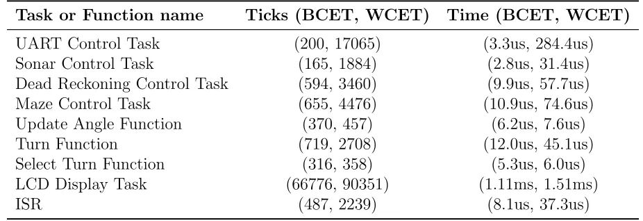
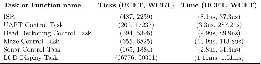
Table 4.2 shows the results summary of each task or function in practical approach we may use for analysis later.
Table 4.2: BCET and WCET using practical approach
Task or Function name Ticks (BCET, WCET) Time (BCET, WCET)
UART Control Task (200, 17065) (3.3us, 284.4us) Sonar Control Task (165, 1884) (2.8us, 31.4us) Dead Reckoning Control Task (594, 3460) (9.9us, 57.7us) Maze Control Task (655, 4476) (10.9us, 74.6us) Update Angle Function (370, 457) (6.2us, 7.6us) Turn Function (719, 2708) (12.0us, 45.1us) Select Turn Function (316, 358) (5.3us, 6.0us) LCD Display Task (66776, 90351) (1.11ms, 1.51ms)
ISR (487, 2239) (8.1us, 37.3us)
4.2
Theoretical Approach
4.2.1
Limitation of Analysis Tool
Table 4.3: Functions we need to measure
Function name Ticks (BCET, WCET) Time (BCET, WCET)
Queue Send Function (1059, 1485) (17.6us, 24.8us) Queue Receive Function (1107, 1435) (18.5us, 23.9us) Enter Critical Section Functon (218, 229) (3.6us, 3.8us) Exit Critical Section Functon (263, 263) (4.4us, 4.4us)
As their names imply, the queue functions are used to handle the queues and the critical functions are used when we want some codes to be executed in a critical section which will disable all the interrupts. We do not use ARMSAT to measure the LCD display function and ISR because it cannot handle these tasks.
4.2.2
Results
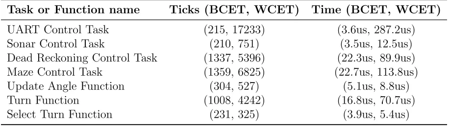
Table 4.4 shows the results summary of each task or function in theoretical approach.
Table 4.4: BCET and WCET using theoretical approach
Task or Function name Ticks (BCET, WCET) Time (BCET, WCET)
4.3
Summary
After comparing the two approaches, we choose the smaller BCET as the final BCET and the longer WCET as the final WCET of each task between the two approaches. Table 4.5 shows the final timing results of each task we need to use in the next chapter.
Table 4.5: Final BCET and WCET of each task
Task or Function name Ticks (BCET, WCET) Time (BCET, WCET)
ISR (487, 2239) (8.1us, 37.3us)
Chapter 5
Analysis and Conclusion
In this chapter we will apply different scheduling approaches to our robot system mainly on the LPC2888 microcontroller and test if the task set is schedulable (meet deadlines) under the certain approach. Based on different approaches, we also try to reduce the microcontroller clock speed to minimum while it is still schedulable.
5.1
Static Scheduling
Since we have an ISR which can be triggered at any time in the system, we cannot use the pure static scheduling method which is without helper interrupts. But we can use the normal static scheduling method with helper interrupts. In this scheduling policy all tasks are in a large loop and each task has the same period, so in order to meet every task’s deadline which equals the period based on our assumptions, the large loop’s period should be less than 3ms which is the minimum period among the five tasks in our case. The next equation from [4] gives us the way to check the schedulability under this approach. Pm is the period of the main loop which equals 3ms. Ci is the execution time
of each task or ISR. Pi is the period of each ISR. Tasks start from 0 to N −1 and ISRs
start from N to N +M −1 assuming that we have N tasks and M ISRs.
i=N−1
X
i=0
Ci+
i=N+M−1
X
i=N
lPm Pi
m Ci
≤Pm (5.1)
After applying our data to the equation, we know thatPi=N−1
i=0 Ci+
Pi=N+M−1
i=N
Pm
Pi
Ci
approach to schedule the five tasks we have. This is probably because the execution time of LCD display task is relatively longer than other tasks comparing to the minimum task period.
5.2
Dynamic Scheduling
Dynamic scheduling means the scheduler can select tasks to run based on different scheduling policies such as static priority assignment and dynamic priority assignment.
We will use some equations in this chapter. In each of these equations, τi means
a periodic task. A set of tasks is represented by τ = {τi} and the tasks are sorted in
non-decreasing order by period. Each τi is associated with (Ti, Di, Ci) which separately
means period, relative deadline and worse case execution time (WCET). We definehp(τi)
as the subset of τ which has tasks with priority equal to or higher than τi.
Before applying different scheduling policies, we need to make some assumptions, because if we do not do this, we cannot ensure the tasks meet their deadlines under all circumstances. These assumptions are also optimistic and they may not be true in practice. But they can help us to analyze problems more efficiently and more easily. Another reason is that all the equations we use to test the schedulability in this chapter are based on these assumptions.
All tasks are periodic
This is why we fix the period of each task in last chapter. We need know the fixed period of each task to do further analysis. If a task’s period length varies during runtime based on different execution times, we choose the fastest possible period.
Deadline of each task equals its period
In our case, the deadline of each task does equal its period. In some cases, if the deadline is shorter than the period, we should use the deadline as the period.
All tasks are independent
line data) dependencies on the UART control task, these tasks are all independent. It is because they cannot block each other which means when dead reckoning control task or maze control task is running and it finds that no data is available (semaphore is not set) from the corresponding queues, it will keep running and exit, so it will not be blocked. This is also why we use semaphore instead of resuming another task in a task when the data is ready.
There is no scheduling overhead
This means we can ignore the time of switching between tasks and the time of context switching. The ISR overhead time is also ignored. Why we do this is because comparing to the shortest deadline, the switching time between tasks or the ISR overhead time is much slower. For safety reason, we need to add some margin to our results because in the real world these scheduling overhead cannot be ignored. We need make to sure our analysis will apply when the robot is running in the real world.
5.2.1
Non-preemptive Scheduling
In non-preemptive scheduling, we do not treat ISR as a task, so in order to get the real execution time of each task, we need to count the ISR execution time in each task. We should also consider the worse case that when a task starts to run, the ISR immediately preempts, so the ISR will preempt for the maximum times when the task is running. We need to add these times back to each task’s WCET. Here the period of ISR we use is the minimum period which is much (20 times) less than the real world period we observe. The system is very safe to use these numbers. We use the following equation to calculate the new WCET. Let LCM denote the lease common multiple of each task’s period that is LCM = [Ci]. N means there are N tasks.
N ewCi =OldCi+
"
dLCM TISRe
Pj=N
j=1
LCM Tj
#
×CISR
Table 5.1: New WCET of each task for non-preemptive scheduling
Task or Function name WCET Ticks WCET Period
UART Control Task 48564 809.4us 3ms Dead Reckoning Control Task 36726 612.1us 4ms Maze Control Task 38160 636.0us 5ms Sonar Control Task 33216 553.6us 40ms LCD Display Task 121930 2032.2us 250ms
ISR 2239 37.3us 86.7us
Rate Monotonic Scheduling
We use the following Theorem 1 and Theorem 2 from [3] to decide if our task set is schedulable or not.
Theorem 1. A periodic task set τ is schedulable using a fixed priority scheduler if and only if
Cmaxi + X
τj∈hp(τi)
jDi Tj
k
Cj ≤Di (5.2)
for ∀τi ∈τ where Cmaxi =max{Ck|k > i}.
Theorem 2. Rate monotonic is an optimal priority assignment for non-preemptively scheduling periodic task sets with Di =Ti.
After applying our task data to Theorem 1, we know that our five tasks all meet the requirement of equation (5.2), so they are schedulable according to Theorem 1. Now we need to figure out what is the minimum microcontroller clock speed we can use so that all the tasks are still schedulable.
We assume that if we reduce the microcontroller clock speed by n times, only each task’s execution time (WCET) will increase by n as new WCET, so the equation in Theorem 1 is changed to:
N ewCmaxi ×n+ X
τj∈hp(τi)
jDi Tj
k
N ewCj ×n≤Di
we apply our five task data to the equation, they all still meet the requirement. After calculation we know the maximum n which is approximate 1.372 since we add some safe margins when calculating, so the minimum clock speed we can get is 60MHz/1.372 = 43.732MHz if we use this RM scheduling approach.
Earliest Deadline First Scheduling
We use the following Corollary 3 from [2] to decide if our tasks set is schedulable or not.
Corollary 3. A periodic task set τ is schedulable using a non-preemptive earliest deadline first scheduler if it satisfies
n
X
i=1
Ci
Ti
≤1 (5.3)
L≥Ci+ i−1
X
j=1
jL−1 Tj
k
Cj (5.4)
for ∀i, 1< i≤n; ∀L, T1 < L < Ti.
After applying our task data to Corollary 3, we know that our five tasks all meet the requirement of equation (5.3) and (5.4), so they are schedulable according to Corollary 3. Now we need to figure out what is the minimum microcontroller clock speed we can use so that all the tasks are still schedulable.
We assume that if we reduce the microcontroller clock speed by n times as before, only each task’s execution time (WCET) will increase by n, so the equation in Corollary 3 is changed to:
n
X
i=1
N ewCi
Ti
×n ≤1 L≥N ewCi×n+
i−1
X
j=1
jL−1 Tj
k
N ewCj ×n
5.2.2
Preemptive Scheduling
From the last chapter, we can get the WCET and WCET ticks of each task sorted by period showing in Table 5.2. Since now we use preemptive scheduling method, we should add ISR as a task, so now we have six tasks in total.
Table 5.2: WCET of each task for preemptive scheduling
Task or Function name WCET Ticks WCET Period
ISR 2239 37.3us 86.7us
UART Control Task 17233 287.2us 3ms Dead Reckoning Control Task 3460 89.9us 4ms Maze Control Task 6825 113.8us 5ms Sonar Control Task 1884 31.4us 40ms LCD Display Task 90351 1510us 250ms
Rate Monotonic Scheduling
We know that if the lowest priority task meets all its deadlines in the worst case, the task set is schedulable, so we use the following equation to estimate the lowest priority task’s response time to determine if it is schedulable.
a0 =Ci+
X
j∈hp(i)
Cj
an+1 =Ci+
X
j∈hp(i)
lan τi
m Cj
For each task set we iterate an until an = an+1. If an ≤ Di, it is schedulable.
Otherwise it is not schedulable.
After applying our tasks data to the equations above, we know that our six tasks all meet the requirement, so they are schedulable.
above is changed to:
a0 =Ci×n+
X
j∈hp(i)
Cj×n
an+1 =Ci×n+
X
j∈hp(i)
lan τi
m
Cj×n
After calculation, from the equations above we can get the maximumnwhich is 1.572, so the minimum clock speed we can get is 60MHz/1.572 = 38.217MHz if we use this RM scheduling approach.
Earliest Deadline First Scheduling
For preemptive EDF scheduling, from [1] we know that periodic task set τ containing m tasks is schedulable if and only if
m X i=1 Ci Ti ≤1
It means if only the microcontroller utilization is less than or equals to 1, the tasks set can be schedulable. In our case, the microcontroller utilization is 0.5785, so it can be schedulable.
We assume that if we reduce the microcontroller clock speed by n times, only each task’s execution time (WCET) will increase by n times at this time, so equation above is changed to:
Xm
i=1
Ci
Ti
×n ≤1
After calculation, from the equation above we can get the maximumnwhich is 1.7286, so the minimum clock speed we can get is 60MHz/1.7286 = 34.710MHz if we use this EDF scheduling approach.
5.3
Conclusion
Table 5.3: Minimum clock speeds summary
Non-preemptive Preemptive
Rate Monotonic 43.732MHz 38.217MHz
Earliest Deadline First 43.732MHz 34.710MHz
From Table 5.3, in non-preemptive scheduling, we see the minimum clock speeds of RM scheduling and EDF scheduling are exactly the same which means that sometimes the schedulabilities of RM scheduling and EDF scheduling are the same according to Theorem 1 and Theorem 2. This is because we assume that the deadline of each task equals its period so that RM scheduling and EDF scheduling are the same in our case. In preemptive scheduling, EDF scheduling is more optimal than RM scheduling. Preemptive scheduling is more optimal than non-preemptive scheduling in both RM scheduling and EDF scheduling.
It is obvious that earliest deadline first in preemptive scheduling is the most optimal when the deadline of each task equals its period in our case.
We also implement the non-preemptive RM scheduling approach in FreeRTOS to show that all tasks can meet their deadlines when the clock runs at lower speeds. In our experiment, we can reduce the clock speed to 24MHz which is much lower than 43.732MHz from our theoretical calculation. This is because the period of ISR we use for theoretical calculation is the minimum period which is much (20 times) less than the real world period we observed. The ISR should be triggered much slower in the real world when the robot is running. The minimum utilization bound of ISR is too high which is 0.4302 in our theoretical calculation, but for safety reason we have to consider the theoretical worst case.
ISR which means we reduce a portion of the utilization bound of a more frequent running task and add a same portion of utilization bound to a relative less frequent running task.
Chapter 6
Future Work
Optimize and enhance the current tasks
The current tasks may not be optimal, so we will try to figure out how to optimize them to achieve much slower microcontroller clock speed under different scheduling policies. As what we have discussed in the last chapter, we can reduce the UART speed to reduce the ISR utilization bound. We can also reduce the execution time of ISR by moving the decoding function to the UART control task.
We will also enhance the dead reckoning algorithm such as adding more strips in the wheel encoder disc to get more accurate wheel rotation information and using a more complicated algorithm to get more accurate results. Building LCD display queues and semaphores to allow more than one task to display data on the LCD may be another thing to do to enhance the LCD control task.
For the sonar control task, we will change the current sonar range finder to a more sensible senor to detect the obstacles. The current sonar range finder cannot distinguish the distance less than 15cm.
Expand new tasks
Work with ARMSAT
Now ARMSAT is not very compatible with our application. In order to get more accurate static timing information of each task for better analysis, based on the limitations of ARMSAT, we may try to help enhance ARMSAT which can work with FreeRTOS and we will use our application to test ARMSAT. We also need to figure out why ARMSAT gives us some inaccurate results in the last chapter, such as why the BCET is longer than that we measure in the real world etc.
Apply stack analysis
REFERENCES
[1] C. L. Liu and James W. Layland Scheduling Algorithms for Multiprogramming in a Hard Real-Time EnvironmentJournal of the ACM, Vol. 20, No.1, pp. 46-61, January 1973.
[2] Kevin Jeffay, Donald F. Stanat and Charles U. Martel On Non-Preemptive Schedul-ing of Periodic and Sporadic Tasks Proceedings of IEEE Real-Time Systems Sym-posium, pp. 129-139, December 1991.
[3] Moonju Park Non-preemptive Fixed Priority Scheduling of Hard Real-Time Periodic Tasks ICCS, Part IV, LNCS 4490, pp. 881-888, 2007.
[4] Philip Koopman Better Embedded System Software Beta Release, pp. 134-138, Jan-uary 2010.
[5] Pololu Corporation Pololu 3pi Robot User’s Guide 2009.
[6] Ibrahim Kamal WFR, a Dead Reckoning Robothttp://www.ikalogic.com/wfr2.php, April 2009.
[7] Dafydd Walters Implementing Dead Reckoning by Odometry on a Robot with R/C Servo Differential Drive http://www.seattlerobotics.org/Encoder/200010/dead -reckoning article.html, September 2000.
[8] Nathaniel Bowditch The American Practical Navigator http://www.irbs.com/bow-ditch, Chap. 7, 1995.
[9] Department of Computer Science, Dortmund University of Technology Overview on Static Timing Analysis http://ls12-www.cs.tu-dortmund.de/research/activities/-wcc/motivation/ta/index.html, June 2010.
[10] Alexander Dean Sharing the Processor: A Survey of Approaches to Supporting Concurrency 2010.
[11] Sangyeol Kang Integrated Development Environment for ARM 2009. [12] NXP Semiconductors LPC2880/LPC2888 User Manual June 2007.
[13] Real Time Engineers Ltd. FreeRTOS Quick Start Guide http://www.freertos.org/-index.html?http://www.freertos.org/FreeRTOS-quick-start-guide.html, 2010. [14] The Department of Electrical and Computer Engineering, The University of the West
[15] Atmel Corporation ATmega48/88/168 Datasheet February 2009. [16] Pololu Corporation Pololu AVR C/C++ Library Users Guide 2009. [17] Pololu Corporation Pololu AVR Library Command Reference 2009. [18] Optrex Corporation LCD Module Specification November 2000. [19] Hitachi Ltd. HD44780U (LCD-II) DatasheetSeptember 1999. [20] MaxBotix Inc. LV-MaxSonar-EZ4 DatasheetJanuary 2007.
Appendix A
Instructions to Build the Robot
A.1
Hardware Parts
3pi Robot
We use the 3pi robot from http://www.pololu.com. The newest version of 3pi robot uses the ATmaga328 microcontroller which may cause a slight difference from what we build in this project.
Odometers
We use two QTR-1A reflectance sensors from http://www.pololu.com. We connect the VIN pins of the sensors to the VCC pins of the 3pi robot, the GND pins of the sensors to the GND pins of the 3pi robot and the OUT pins of the sensors to the ADC6 pin and the ADC7 pin of the 3pi robot respectively. Then we can use the ATmega168 microcontroller to control the sensors. [21] provides more information about the QTR-1A reflectance sensor.
LPC-H2888 Board
the PD1 pin and the PD0 pin of the 3pi robot respectively. Then we can communicate between the two parts.
LCD
We use the LCD from the original 3pi robot. [12] and [18] provide the information about how to connect the LCD to the LPC-H2888 board through the LCD interface. Then we can use the LPC2888 microcontroller to control the LCD. [19] provides more information about the LCD.
Sonar Range Finder
We use the Maxbotix LV-MaxSonar-EZ4 sonar range finder from http://www.pololu.com. Then we connect the VCC pin, the GND pin and the AN pin of the sonar range finder to the VREF(DADC) pin, the VCOM(DADC) pin and the AIN0 pin of the LPC-H2888 board respectively. We also need to connect the VREF(DADC) pin and the VCOM(DADC) pin to the SUPPLY 3.3V pin and the GND pin respectively. Then we can use the LPC2888 microcontroller to control the sonar range finder. [20] provides more information about the sonar range finder.