Multi-model ensembling of probabilistic streamflow forecasts: Role of predictor state space in skill evaluation

Multi-model Ensembling of Probabilistic Streamflow Forecasts: Role of Predictor State Space in skill evaluation

Institute of Statistics Mimeo Series 2595

A.Sankarasubramanian1, Naresh Devineni1 and Sujit Ghosh2

1

Department of Civil Engineering, North Carolina State University, Raleigh, NC 27695-7908. 2

Department of Statistics, North Carolina State University, Raleigh, NC 27695-8203.

ABSTRACT

Seasonal streamflow forecasts contingent on climate information are essential for short-term planning and for setting up contingency measures during extreme years. Recent research shows that operational climate forecasts obtained by combining different General Circulation Models (GCM) have improved predictability/skill in comparison to the predictability from single GCMs [Rajagopalan et al., 2002; Doblas-Reyes et al., 2005]. In this study, we present a new approach for developing multi-model ensembles that combines streamflow forecasts from

various models by evaluating their performance from the predictor state space. Based on this, we show that any systematic errors in model prediction with reference to specific predictor

contingent on SSTs, the methodology gives higher weights in drawing ensembles from a model that has better predictability under similar predictor conditions. The performance of the multi-model forecasts are compared with the individual multi-model’s performance using various forecast verification measures such as anomaly correlation, root mean square error (RMSE), Rank Probability Skill Score (RPSS) and reliability diagrams. By developing multi-model ensembles for both leave-one out cross validated forecasts and adaptive forecasts using the proposed methodology, we show that evaluating the model performance from predictor state space is a better alternative in developing multi-model ensembles instead of combining model’s based on their predictability of the marginal distribution.

1.0

INTRODUCTION

statistical relationship [Robertson et al. 2004, Landman and Goddard, 2002; Gangopathyaya et al.,2005] or develop a low dimensional model that relates the observed streamflow/reservoir inflow to climatic precursors such as El Nino Southern Oscillation (ENSO) conditions [Hamlet and Lettenmaier, 1999; Souza and Lall, 2003; Sankarasubramanian and Lall, 2003]. Seasonal streamflow forecasts obtained using these approaches are represented probabilistically using ensembles to quantify the uncertainty in prediction which primarily arises from both changing boundary conditions (SST) and initial conditions (atmospheric and land surface conditions). Apart from the uncertainties resulting from initial and boundary conditions, the model that is employed for developing streamflow forecasts could also introduce uncertainty in prediction. In other words, even if the streamflow forecasting model is obtained with observed boundary and initial conditions (perfect forcings), it is inevitable that the simulated streamflows will have uncertainty in prediction, which is otherwise known as model error/uncertainty. One approach to reduce model uncertainty is through refinement of parameterizations and process representations in GCMs. Given that developing and running GCMs is time consuming, recent efforts have focused in reducing the model error by combining multiple GCMs to issue monthly climate forecasts [Rajagopalan et al., 2002; Robertson et al., 2004; Barnston et al., 2003; Doblas-Reyes et al., 2000; Krishnamurthi et al., 1999]. Thus, combining forecasts from multiple models seems to be a good alternative in improving the predictability of large scale GCM fields, which could in turn improve predictability from both dynamically downscaled streamflow forecasts as well as statistically downscaled forecasts.

predictability conditioned on the predictor state space. The primary reason for better performance of multi-model ensembles is in incorporating realizations from various models, thereby increasing the number of ensembles to represent conditional distribution of climatic attributes. Recent studies on improving seasonal climate forecasts using optimal multi-model combination techniques basically assign weights for a particular model based on its ability to predict the marginal distribution of the climatic variable [Rajagopalan et al., 2002; Robertson et al., 2004; Barnston et al., 2003]. In other words, GCMs with better predictability in a particular month/season will have higher proportion of ensembles represented in the multi-model forecasts. Given that each model’s predictability could also vary depending on the state of the predictor (SSTs for GCMs), we develop a new methodology for multi-model ensembling that assigns weights to each model by assessing the skill of the models contingent on the predictor state. The proposed methodology is employed upon two low dimensional seasonal streamflow forecasting models that use tropical Pacific and Atlantic SST conditions to develop multi-model ensembles of streamflow forecasts. Though the proposed approach is demonstrated by combining two statistical streamflow forecasting models, we believe that the approach presented in section 3.2 can be extended to combine multiple GCMs. Since the streamflow forecasts are represented probabilistically, we use Rank Probability Score (RPS) [Candile and Talagrand, 2005] as a measure to assess the model’s predictability.

probabilistic streamflow forecasts for predicting the summer flows (July-August-September, JAS) into Falls Lake, Neuse river basin NC. Finally, we show the application of the proposed multi-model ensembling in Section 3 to develop improved probabilistic streamflow forecasts for predicting JAS inflows into the Falls Lake, NC along with discussions for applying the proposed methodology for combining GCM forecasts.

2.0 BACKGROUND

climatology as one of the forecasts is also a viable option, particularly when the actual outcome is beyond the predictability of all models [Rajagopalan et al., 2002; Robertson et al., 2004].

develop a multi-model ensembling scheme that formally assesses and compares the skill of the model with other competing models under any given predictor conditions so that lower weights are assigned for a model that has poor predictability under those conditions. The next section formally develops a multi-model ensembling scheme using Rank Probability Score (RPS) as the basic measure for evaluating the forecasting skill. Though we apply this approach for combining two statistical streamflow forecasting models with climatology, this could be even extended to combine ensembles from multiple GCMs.

3.0 Multi-Model Ensembling based on Predictor State: Methodology Development

both predictors will always lead to poor prediction particularly when the first predictor is below the threshold value (Figure 1b). Thus, our approach of multi-model ensembling gives emphasis for assessing the model performance based on the boundary conditions, the predictor state. For instance, if the predictability of all models is really bad during a particular condition, then one would replace model forecasts with climatology by assigning higher weights for climatological ensembles, which are typically generated by simple bootstrapping of the observed flow values. In the next section, we formally describe the multi-model ensembling procedure that could be employed upon a given set of forecasts and the predictors that influence those forecasts.

3.2 Multi-Model Ensembling based on Predictor State Space - Algorithm

Let us suppose that we have streamflow forecasts,Qim,t, where m=1,2..,M denoting the

forecasts from ‘M’ different models, i = 1,2, ..N representing ensembles of the conditional distribution of streamflows with ‘N’ denoting the total number of ensembles and‘t’ denoting the time (season/month) for which the forecast is issued. Assuming that we have a total of t= 1,2,...n years for which both the retrospective forecasts,Qim,t, are available from ‘M’ different models and

probabilistic forecasts using Rank Probability Score (RPS) [Murphy 1970, Candille and Talagrand 2005, Anderson, 1996]. The Rank Probability Skill Score (RPSS) represents the level of improvement of the RPS in comparison to the reference forecast strategy which is usually assumed to be climatology. Appendix A provides a brief introduction on obtaining RPS and RPSS for a given probabilistic forecasts.

Let us denote the RPS and RPSS of the probabilistic forecasts,Q_im_,t, for each time step

asRPS_tm,RPSS_tm. Our approach to assess the skill of the model is by looking at its ability to

predict under similar climatic conditions or the predictor state, which could be identified by choosing a distance metric that computes the distance between the current predictor state, Xt and the historical predictor vector X. One could use simple Euclidean distance or a more generalized distance measure such as Mahalonobis distance metric, which is more useful if the predictors’ exhibit correlation among them. Compute the distances dtl between the current conditioning state Xt, and the historical predictor vector Xl as

) (

ˆ ) (

d_tl = X_t −X_l T ∑−1 X_t − X_l ... (1)

where ∑ˆ denotes the variance-covariance matrix of the historical predictor vector X. One can note that if l=t the distance metric, dtl, reduces to zero. Using the distance vector d, identify the ordered set of nearest neighbor indices J. Thus, jth element in the distance vector metric provides the jth closest Xl to the current state Xt. Using this information, we assess the performance of each model in the predictor state space as

∑

=

λ K

j

m j

RPS

K 1

) ( m

K t,

1

... (2)

average skill of the forecasting model, m, by choosing ‘K’ years that resemble very similar to the current condition, Xt. Using λmt,K obtained for each model at each time step, we obtain the weights for multi-model ensembling so that models with better performance during a particular climatic conditions needs to be represented with more number of ensembles in comparison to a model with lower predictability under those conditions. It is important to note RPS is a measure of error in predicting the probabilities.

∑

λ λ = _M

m m

K t m

K t m

K t

w

1 , , ,

/ 1 / 1

... (3)

If λmt,K is zero for a subset of models M1≤ M, then the weights

m K t

w, are distributed equally

between the models for which λmt,K is zero with the rest of models weights being equal to zero.

The multi-model forecasts for each time step could be developed by drawing w_tm_,K *Nensembles

from each model to constitute the multi-model ensembles. Thus, one has to specify the number of neighbors ‘K’ to implement this approach. It is also important to note that choosing fewer ‘K’ relates to evaluating the model performance over few years of similar conditions, which does not imply that the forecasts are developed from the predictands and predictors from the identified similar conditions alone. In fact, Qim,t are forecasts developed based on the observed values of the

predictand and predictand over a particular training period (For leave-one out cross validated forecasts, we use ‘n-1’ years of record as training period; For adaptive forecasts, we use 60 years of observed record from 1928-1986 as the training period). Thus, we use the weights, w_tm_,K, only

to draw the ensembles from Qim,t, not to develop the conditional distribution itself. The simplest

ensembles over n years of record. We evaluate two different strategies in choosing the number of neighbors ‘K’ to develop multi-model ensembles. The performance of multi-model ensembles is also compared with individual model’s predictability using various verification measures such as average RPS, average RPSS, anomaly correlation and root mean square error (RMSE).

4.0 Seasonal Streamflow Forecasts Development for the Neuse Basin

For the purpose of demonstrating the proposed multi-model approach in Section 3, we first develop probabilistic seasonal streamflow forecasts using climate information for the Falls Lake, Neuse river basin in North Carolina (NC). We develop streamflow forecasts using two statistical models, one based on parametric regression model and another using a nonparametric approach based on resampling [Souza and Lall, 2003] using SST conditions from tropical Pacific, North Atlantic and NC coast. We first provide baseline information for the Neuse basin and its importance to the water management of the research triangle area of NC.

4.1 Baseline Information for the Neuse basin (Figure 3)

maintaining the operational rule curve at 251.5 is very challenging during those months. The following section provides a quick overview of climate and streamflow teleconnection in the US with specific focus on the South Eastern US.

4.2 Climate and Streamflow Teleconnection in the US – Brief Overview

SST conditions in the tropical Pacific and tropical Atlantic to develop seasonal streamflow forecasts into Falls Lake during July-September (JAS).

4.3 Seasonal Streamflow Forecasts Development – Individual Models

Seasonal streamflow forecasts based on climate information could be developed by downscaling climate forecasts from GCMs to streamflow or by developing a low dimensional model that relates conditional distribution of streamflows to the climatic precursors. The difficulty in utilizing GCM predicted fields to develop streamflow forecasts at

regional/watershed scale is due to the availability of information at larger spatial scales

(2.5°×2.5°) and requires nesting of models of various spatial resolution by downscaling the GCM precipitation and temperature forecasts through a Regional Climate Model (RCM) (60 Km× 60Km) whose finer spatial scale information could be given as inputs into a sub grid-scale hydrologic model to develop forecasts of streamflow [Leung et al., 1999; Roads et al., 2003, Yu et al., 2002; Nobre et al., 2001]. An alternative would be to develop statistical model that relates the climatic conditions with the streamflow at a particular site [Souza and Lall, 2003;

Sankarasubramanian and Lall, 2003].

Our objective is to estimate the conditional distribution of streamflows, f(Qt|Xt), that is going to occur in the upcoming season based on the climatic conditions Xt using the chosen statistical model. The estimate of the conditional distribution in the ensemble as specified in section 3 as Qim,t with ‘t’ denoting the time, ‘i’ representing the ensemble and ‘m’ denoting the

model. Based on the observed streamflow, Qt and the predictorsXt =

[

]

(e.g., log normal) for the conditional distribution or by using a data driven approach which estimates the conditional distribution using nonparametric techniques such as resampling. For the parametric approach, we employ regression model by assuming the flows follows a lognormal distribution and estimate the conditional mean and standard deviation of the lognormal

parameters. Using the lognormal parameters, we generate ensembles from lognormal distribution and transform it back into the original space to represent the conditional distribution of

flows,Qim,t. The other approach we employ is the semi-parametric resampling algorithm of Souza

and Lall [2003]. The main advantage of this approach is that it does not specify any functional form for estimating the conditional distribution, thus allowing the data to describe the conditional distribution of streamflows. For further details, see Souza and Lall [2003].

4.3.1 Diagnostic Analyses, Predictor Identification and Dimension Reduction

To identify predictors that influence the streamflow into Falls Lake during JAS, we consider SST conditions during April-June (AMJ) which are available from IRI data library (http://iridl.ldeo.columbia.edu/expert/ SOURCES/.KAPLAN/.EXTENDED/.ssta). Figure 3b shows the spearman rank correlation between the observed streamflow during JAS at the Falls Lake and the SST conditions during AMJ. From Figure 3b, we see clearly that SST over ENSO region (170E - 90W and 5S - 5N), the North Atlantic region (80W- 40W and 10N - 20N), and the NC Coast region (75W- 65W and 22.5N- 32.5N) influence the summer flows into Falls Lake. It is important to note that we consider SST regions whose correlations are significant and greater than the threshold value of ±1.96/ n−3 where ‘n’ is to the total number years (n=75 years for Falls Lake) of observed records used for computing the correlation.

orthogonal function (EOF) analysis, on the predictors (SST fields) could also be performed by singular value decomposition (SVD) on the correlation matrix or covariance matrix of the predictors. Since PCA is scale dependent, loadings (Eigen vectors or EOF patterns) obtained from covariance matrix and correlation matrix are different. Importance of each principal component is quantified by the fraction of the variance the principal component represents with reference to the original predictor variance, which is usually summarized by the scree plot. Detailed comparisons on the performance of correlation matrix and covariance matrix based PCA to find coupled patterns are discussed in Bretherton et al., [1992] and Wallace et al., [1992]. Mathematics of PCA and the issues in selecting the number of principal components using scree plot could be found in Dillon and Goldestein [1984], Wilks [1995], Von storch and Zweiers [1998]. Figure 3c shows the percentage of variance explained by each principal component and the first two components account for 72% of the total variance shown in the predictor field in Figure 3b. Based on the eigenvectors obtained from PCA (figure not shown), the first component representing the ENSO region has correlation of 0.36 with observed streamflow and the second component representing the Atlantic has a correlation of -0.23 (significance level +/- 0.21 for 75 years of record) with the inflows at Falls Lake. We employ these two principal components to develop seasonal streamflow forecasts for JAS for the Falls Lake.

4.3.2 Performance of Individual Forecasting Models – Resampling and Regression Approach

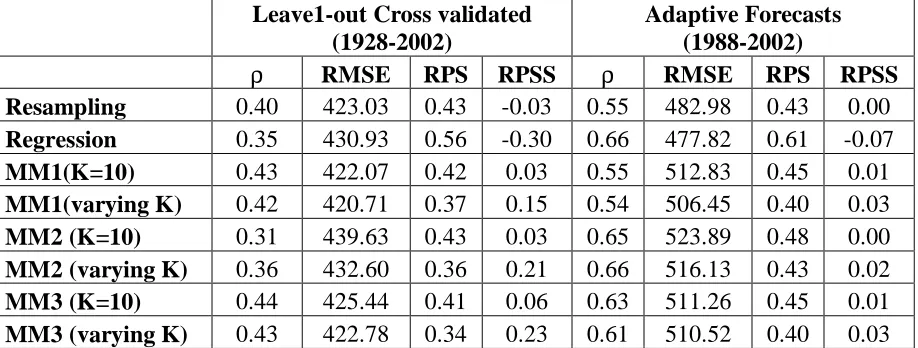
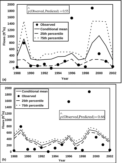
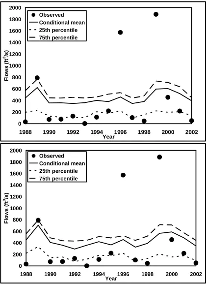
predictors from the observed data set (Qt, Xt, t =1,2,…,n) for the validating year and the forecasts are developed using the rest of the (n-1) observations, where n is the total length of observed records in a given site. For instance, to develop retrospective leave-1 out forecasts from regression model, a total of ‘n’ regression models is developed by leaving out the observation of the validating years. By employing the developed forecasting model with (n-1) observations, the left out observation (Q-t, with -t denoting the left out year or the validating year) is predicted by using the state of the predictor/principal components (X-t,) in the validating year. Table 1 gives various performance measures of the probabilistic forecasts from both models. To develop adaptive streamflow forecasts, we use the observed streamflow and the two dominant principal components from 1928-1987 to predict the streamflow for 15 year period from 1988-2002. Figure 4 shows the adaptive streamflow forecasts for both parametric regression and the semi-parametric models. It is important to note the forecasts are probabilistic represented probabilistically in the form of ensembles. The correlation between the observed streamflows and the ensemble mean of the cross validated forecasts for regression and resampling approach is 0.40 and 0.35 respectively, which is significant for the 75 years of observed record. The correlation between the observed streamflows and the ensemble mean of the adaptive forecasts is 0.66 and 0.55 for regression and resampling approach respectively. Table 1 also shows other verification measures such as RPS, RPSS and Root Mean Square Error (RMSE) for both adaptive and leave-1 out cross validated forecasts for both models. Since the correlations between observed and ensemble mean is significant for both models under leave-1 out cross validated forecasts and adaptive forecasts. We employ both these models for developing multi-model ensembles, which we hope to improve the skill of the individual multi-model forecasts.

In this section, we plan to employ the multi-model ensembling algorithm discussed in section 3.2 to combine the forecasts from individual models along with climatology. The motivation in considering climatology as one of the candidates is upon the presumption that if the observation/outcome falls outside the scope of all the models under certain predictor conditions, then climatology should be preferred over model forecasts. Recent studies have shown that combining individual models with climatology at one step results with one model getting all the weight (equal to one) leaving the rest’s weight to zero, primarily due to the high dimensionality of the optimization space [Rajagopalan et al., 2002; Robertson et al., 2004]. A two step procedure of combining individual model with climatology and then combining the resulting probabilistic forecasts from the combination of individual models with climatology gives more robust weights and results in improved predictability [Robertson et al., 2003; Goddard et al., 2003]. We also perform a two step procedure in developing multi-model ensembles by first combining the probabilistic forecasts from regression model and resampling model separately with climatology and then combining the resulting forecasts from ‘M’ combinations to develop one single multi-model forecasts. We also choose the number of neighbors K in equation 3.2 by two different methods to identify the relevant predictor condition: (a) by selecting a fixed ‘K’ for all the years, (b) Varying Kt each year such that the selected ‘Kt’ corresponds to the minimum RPS that could be obtained from the multi-model forecasts. This will help us to understand the role of choosing the number of neighbors in developing multi-model ensembles proposed in section 3.2.

5.1 Skill of the Individual Models from Predictor state space

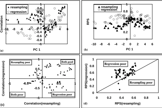
appropriate weights based on (3) for all the models to develop multi-model ensembles. To generalize this further, by considering climatological ensembles itself as a forecast we intend to give higher weights to climatology if the predictability of all the models is poor under a particular predictor condition. By analyzing the predictability of the two candidate streamflow forecasts shown in figure 4 for JAS into Falls Lake based on the dominant predictor, PC1, we show the predictability of each model in Figure 5 principal component (represents primarily ENSO conditions) by choosing ten neighboring conditions for estimating two verification measures, correlation and RPS. As one can see from Figure 5a, one may prefer to choose forecasts from resampling model instead of forecasts from parametric regression particularly when the dominant principal component, PC1 is less than -2, since the predictive ability of regression model is negative during those conditions. This is seen in Figure 5b with the RPS of resampling lesser than that of RPS of regression. Figures 5c and 5d show the relative performance of both models against each other. From figure 5c, we can see that one would prefer climatological ensembles would be preferred particularly when correlations estimated from the neighborhood on both models are negative. From 5d, we can see similar conditions corresponding to PC1 being negative with RPS score of regression model being higher than that of RPS of resampling. Thus, the multi-model ensembling algorithm in section 3.2 identifies these conditions based on RPS using (2) and develops a general procedure for multi-model ensembling based on the algorithm in section 3.2. In the next two sections, we present the performance of multi-model forecasts based on two different strategies of choosing the number of neighbors over which the performance of the models are evaluated.

important to note that the improved performance of multi-model ensembles is seen in almost all evaluation measures. Even with fixed number of neighbors, the multi-model ensembling algorithm based on predictor state space provides improved predictability than the individual model forecasts. Ideally, one would like to have the number of neighbors varying each year so that model predictability is evaluated depending on the predictor conditions. For instance, under extreme conditions of PC1, one would like to choose small ‘K’ since they correspond to similar predictor conditions. To understand whether we see any relationship between the chosen Kt for every year that corresponds to the minimum RPS of the multi-model ensembles, we plot the optimized Kt with PC1 in figure 7. From figure 7, we see clearly that few number of neighbors is chosen particularly if the PC1 corresponds to above normal or below normal values. It is important to note that PC1 primarily denotes ENSO conditions (correlation between PC1 and Nino3.4 = 0.36), thus positive PC1 denoting the El Nino and negative conditions denoting La Nina. Though we may consider K =1 in evaluating the skill of the model in predictor state space (2), it does not imply that the forecast for that particular year is drawn from only one year. Instead, the algorithm in section 3.2 gives smaller weights to the model that has higher RPS, thus drawing fewer ensembles from that individual model’s probabilistic forecasts, which actually depends on the training data set (For adaptive forecasts, it is 1928-1987 streamflow values and for retrospective leave-1 cross validated forecasts, it is 1928-2002 except the observed flow in the year for which the forecast is developed). Thus, the multi-model scheme in section 3.2 only gives weights for a particular model to draw ensembles based on its predictive ability in the predictor state space, but the probabilistic forecasts that constitute the ensembles from individual models are derived based on the observed streamflows available for fitting.

6.0 Summary and Conclusions

A new approach for developing multi-model ensembles is developed and verified by combining streamflow forecasts from two statistical models. The approach develops multi-model ensembles by assessing the predictability of the model contingent on the predictor conditions. This is carried out by identifying similar conditions from the current state of the predictor by choosing a either fixed or varying number of neighbors K and assessing the performance of the model over those neighbors using average RPS. The average RPS over K neighbors are converted into weights for each models which were then employed to draw appropriate (proportional to weights) number of ensembles to develop multi-model ensembles. The proposed approach was tested in combining two low dimensional statistical models to develop multi-model ensembles of JAS streamflow forecasts. By comparing the performance of multi-multi-model ensembles with individual model performance using various verification measures as well as with leave-1 out cross validated forecasts and adaptive forecasts, we show that the proposed approach significantly improves the predictability of seasonal streamflow forecasts into Falls Lake of the Neuse River basin, NC.

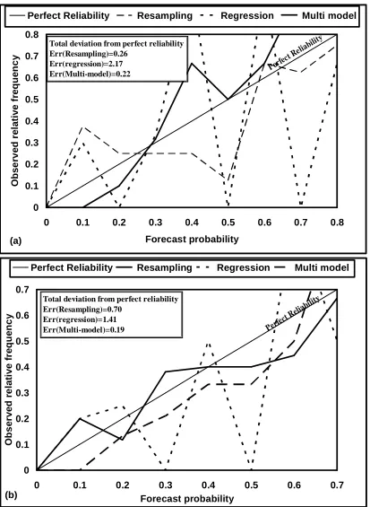
the models is poor under a particular condition, then our approach will eventually replace the multi-model ensembles with only climatological ensembles. This ensures significant reduction in false alarm and missed targets in the issued forecasts and results in better reliability between the forecasted probability and the corresponding observed relative frequency. Further, the approach may use very small/fixed number of neighbors in assessing the predictability of model in the predictor state space, but the average skill of the model in those conditions are only used to arrive at the weights which are employed to draw appropriate multi-model ensembles. Thus, the developed multi-model forecasts essentially contain the combined forecasts from individual model forecasts, which are obtained based on the training period utilized from the observed records of streamflows and predictors. Thus, small number of neighbors used to obtain weights should not be interpreted as that many number of years of record were employed for developing the multi-model forecasts. Though the approach requires a common predictor across all the ‘M’ models considered for combination, one can easily identify the dominant predictor that will be common across the predictors of all the models by using dimension reduction techniques. For instance, if the same approach were to be employed for combining multiple GCMs, we can utilize the dominant principal components of the underlying predictors, SSTs that influence the precipitation and streamflow potential of that region. Our future studies will investigate on combining multiple GCMs to develop multi-model ensembles of precipitation forecasts, using which one can obtain seasonal streamflow forecasts by employing any of the discussed downscaling techniques.

Appendix A: Rank Probability Score and Rank Probability Skill Score

some measures of central tendency such as mean or median of the conditional distribution, which do not give any credit to the probabilistic information in the forecast. Rank Probabilistic Skill Score (RPSS) computes the cumulative squared error between the categorical forecast

probabilities and the observed category relative to some reference forecast (Wilks, 1995). Here

category represents dividing the climatological/observed streamflow, Q, into d=1,2,...,D

divisions and expressing the marginal probabilities as Pd(Q). Typically, the divisions are made

equal probabilistically with O=3 categories known as terciles with each category having 1/3

probability of occurrence. These three categories are known as below normal, normal and

above-normal whose end points provide streamflow values corresponding to the particular category.

Thus, for a total of D categories, the end points based on climatological observations for dth

category could be written as Qd, Qd+1 (For d=1, Q1= 0; d=D; QD+1 = Qmax). Given streamflow

forecasts at time‘t’ from mth model with i=1, 2... N ensembles,Qim,t, then the forecast probabilities

for the dth category could be expressed as FP Q nm N

t d m

t

d,( )= , / by computing the number of ensembles between Qd≤Qim,t≤ Qd+1.To compute RPSS, the first step is to compute Rank

Probability Score (RPS). Given D categories and FP, (Q)

m t

d for a forecast, we can express the RPS

for a particular year‘t’ from mth model as

[

]

∑

t CF CO

RPS

1

2

, ...(A-1)

where

∑

= = d q m t d m t d FP CF 1 ,

, is the cumulative probabilities of forecasts up to category d and COd is

RPS, we can compute RPSS for a reference forecast, which is usually the climatological forecasts that have equal probability of occurrence in each category FPdct (Q) 1/D

lim

, = .

lim

1 _c

t m t m

t

RPS RPS

RPSS = − ...(A-2)

REFERENCES

Anderson, J. L. (1996), A method for producing and evaluating probabilistic forecasts from ensemble model integrations, Journal of Climate, 9, 1518-1530.

Barnston AG, Mason SJ, Goddard L, DeWitt DG, Zebiak SE. Multimodel ensembling in seasonal climate forecasting at IRI. Bulletin of the American Meteorological Society 2003;84(12):1783-+.

Brankovic, C., and T. N. Palmer (2000), Seasonal skill and predictability of ECMWF PROVOST ensembles, Quarterly Journal of the Royal Meteorological Society, 126, 2035-2067.

Bretherton CS, Smith C, Wallace JM. An Intercomparison of Methods for Finding Coupled Patterns in Climate Data. Journal of Climate 1992;5(6):541-560.

Candille G, Talagrand O. Evaluation of probabilistic prediction systems for a scalar variable. Quarterly Journal of the Royal Meteorological Society 2005;131(609):2131-2150.

Carpenter, T.M., Georgakakos, K.P., 2001. Assessment of Folsom lake response to historical and potential future climate scenarios. 1. Forecasting. Journal of Hydrology 249, 148–175.

Cayan DR, Redmond KT, Riddle LG. ENSO and hydrologic extremes in the western United States. Journal of Climate 1999;12(9):2881-2893.

Dillon, W. and M. Goldstein, Multivariate Analysis: Methods and Applications. Wiley & Sons, 1984.

Doblas-Reyes FJ, Deque M, Piedelievre JP. Multi-model spread and probabilistic seasonal forecasts in PROVOST. Quarterly Journal of the Royal Meteorological Society

2000;126(567):2069-2087.

Doblas-Reyes FJ, Hagedorn R, Palmer TN. The rationale behind the success of multi-model ensembles in seasonal forecasting - II. Calibration and combination. Tellus Series a-Dynamic Meteorology and Oceanography 2005;57(3):234-252.

Gangopadhyay S, Clark M, Rajagopalan B. Statistical downscaling using K-nearest neighbors. Water Resources Research 2005;41(2).

Georgakakos, KP. Probabilistic climate-model diagnostics for hydrologic and water resources impact studies. Journal of Hydrometeorology 2003;4(1):92-105.

Georgakakos KP, Hudlow MD. Quantitative Precipitation Forecast Techniques for Use in Hydrologic Forecasting. Bulletin of the American Meteorological Society 1984;65(11):1186-1200.

Goddard, L., A. G. Barnston, and S. J. Mason (2003), Evaluation of the IRI's "net assessment" seasonal climate forecasts 1997-2001, Bulletin of the American Meteorological Society, 84, 1761-+.

Goddard L, Barnston AG, Mason SJ. Evaluation of the IRI's "net assessment" seasonal climate forecasts 1997-2001. Bulletin of the American Meteorological Society 2003;84(12):1761-+.

Goddard L, Mason SJ, Zebiak SE, Ropelewski CF, Basher R, Cane MA. Current approaches to seasonal-to-interannual climate predictions. In: International Journal of Climatology; 2001. p. 1111-1152.

Guetter AK, Georgakakos KP. Are the El Nino and La Nina predictors of the Iowa River seasonal flow? Journal of Applied Meteorology 1996;35(5):690-705.

Hagedorn R, Doblas-Reyes FJ, Palmer TN. The rationale behind the success of multi-model ensembles in seasonal forecasting - I. Basic concept. Tellus Series a-Dynamic Meteorology and Oceanography 2005;57(3):219-233.

Hamlet AF, Lettenmaier DP. Columbia River streamflow forecasting based on ENSO and PDO climate signals. Journal of Water Resources Planning and Management-Asce

1999;125(6):333-341.

Hansen JW, Hodges AW, Jones JW. ENSO influences on agriculture in the southeastern United States. Journal of Climate 1998;11(3):404-411.

Kiehl JT, Hack JJ, Bonan GB, Boville BA, Williamson DL, Rasch PJ. The National Center for Atmospheric Research Community Climate Model: CCM3. Journal of Climate

1998;11(6):1131-1149.

Krishnamurti, T. N., C. M. Kishtawal, T. E. LaRow, D. R. Bachiochi, Z. Zhang, C. E. Williford, S. Gadgil, and S. Surendran (1999), Improved weather and seasonal climate forecasts from multimodel superensemble, Science, 285, 1548-1550.

Landman WA, Goddard L. Statistical recalibration of GCM forecasts over southern Africa using model output statistics. Journal of Climate 2002;15(15):2038-2055.

Lecce SA. Spatial variations in the timing of annual floods in the southeastern United States. Journal of Hydrology 2000;235(3-4):151-169.

Leung LR, Hamlet AF, Lettenmaier DP, Kumar A. Simulations of the ENSO hydroclimate signals in the Pacific Northwest Columbia River basin. Bulletin of the American Meteorological Society 1999;80(11):2313-2329.

Mason SJ, Mimmack GM. Comparison of some statistical methods of probabilistic forecasting of ENSO. Journal of Climate 2002;15(1):8-29.

Nobre P, Moura AD, Sun LQ. Dynamical downscaling of seasonal climate prediction over nordeste Brazil with ECHAM3 and NCEP's regional spectral models at IRI. Bulletin of the American Meteorological Society 2001;82(12):2787-2796.

Murphy, A. H. (1970), Ranked Probability Score and Probability Score - a Comparison, Monthly

Weather Review, 98, 917-&.

Palmer TN, Brankovic C, Richardson DS. A probability and decision-model analysis of PROVOST seasonal multi-model ensemble integrations. Quarterly Journal of the Royal Meteorological Society 2000;126(567):2013-2033.

Piechota TC, Dracup JA. Drought and regional hydrologic variation in the United States: Associations with the El Nino Southern Oscillation. Water Resources Research 1996;32(5):1359-1373.

Quan, X., M. Hoerling, J. Whitaker, G. Bates, and T. Xu (2006), Diagnosing sources of US seasonal forecast skill, Journal of Climate, 19, 3279-3293.

Shukla, J., J. Anderson, D. Baumhefner, C. Brankovic, Y. Chang, E. Kalnay, L. Marx, T. Palmer, D. Paolino, J. Ploshay, S. Schubert, D. Straus, M. Suarez, and J. Tribbia (2000), Dynamical seasonal prediction, Bulletin of the American Meteorological Society, 81, 2593-2606.

Rajagopalan B, Lall U, Zebiak SE. Categorical climate forecasts through regularization and optimal combination of multiple GCM ensembles. Monthly Weather Review

Rasmusson EM, Carpenter TH. Variations in Tropical Sea-Surface Temperature and Surface Wind Fields Associated with the Southern Oscillation El-Nino. Monthly Weather Review 1982;110(5):354-384.

Regonda SK, Rajagopalan B, Clark M, Zagona E. A multimodel ensemble forecast framework: Application to spring seasonal flows in the Gunnison River Basin. Water Resources Research 2006;42(9).

Rhome JR, Niyogi DS, Raman S. Mesoclimatic analysis of severe weather and ENSO interactions in North Carolina. Geophysical Research Letters 2000;27(15):2269-2272.

Roads J, Chen S, Cocke S, Druyan L, Fulakeza M, LaRow T, et al. International Research Institute/Applied Research Centers (IRI/ARCs) regional model intercomparison over South America. Journal of Geophysical Research-Atmospheres 2003;108(D14).

Robertson AW, Kirshner S, Smyth P. Downscaling of daily rainfall occurrence over northeast Brazil using a hidden Markov model. Journal of Climate 2004;17(22):4407-4424.

Robertson AW, Lall U, Zebiak SE, Goddard L. Improved combination of multiple atmospheric GCM ensembles for seasonal prediction. Monthly Weather Review 2004;132(12):2732-2744.

Ropelewski CF, Halpert MS. Global and Regional Scale Precipitation Patterns Associated with the El-Nino Southern Oscillation. Monthly Weather Review 1987;115(8):1606-1626.

Sankarasubramanian A, Lall U. Flood quantiles in a changing climate: Seasonal forecasts and causal relations. Water Resources Research 2003;39(5).

Schmidt N, Lipp EK, Rose JB, Luther ME. ENSO influences on seasonal rainfall and river discharge in Florida. Journal of Climate 2001;14(4):615-628.

Seo DJ, Koren V, Cajina N. Real-time variational assimilation of hydrologic and hydrometeorological data into operational hydrologic forecasting. Journal of Hydrometeorology 2003;4(3):627-641.

Shukla, J., J. Anderson, D. Baumhefner, C. Brankovic, Y. Chang, E. Kalnay, L. Marx, T. Palmer, D. Paolino, J. Ploshay, S. Schubert, D. Straus, M. Suarez, and J. Tribbia (2000), Dynamical seasonal prediction, Bulletin of the American Meteorological Society, 81, 2593-2606.

Souza FA, Lall U. Seasonal to interannual ensemble streamflow forecasts for Ceara, Brazil: Applications of a multivariate, semiparametric algorithm. Water Resources Research 2003;39(11).

Stephenson, D. B., C. A. S. Coelho, F. J. Doblas-Reyes, and M. Balmaseda (2005), Forecast assimilation: a unified framework for the combination of multi-model weather and climate predictions, Tellus Series a-Dynamic Meteorology and Oceanography, 57, 253-264.

Trenberth KE, Guillemot CJ. Physical processes involved in the 1988 drought and 1993 floods in North America. Journal of Climate 1996;9(6):1288-1298.

Wallace JM, Smith C, Bretherton CS. Singular Value Decomposition of Wintertime Sea-Surface Temperature and 500-Mb Height Anomalies. Journal of Climate 1992;5(6):561-576.

Wilks, D.S., Statistical Methods in the Atmospheric Sciences, Academic Press, 1995.

Wood AW, Kumar A, Lettenmaier DP. A retrospective assessment of National Centers for Environmental Prediction climate model-based ensemble hydrologic forecasting in the western United States. Journal of Geophysical Research-Atmospheres 2005;110(D4).

Wood AW, Maurer EP, Kumar A, Lettenmaier DP. Long-range experimental hydrologic forecasting for the eastern United States. Journal of Geophysical Research-Atmospheres 2002;107 (D20).

Yu Z, Barron EJ, Yarnal B, Lakhtakia MN, White RA, Pollard D, et al. Evaluation of basin-scale hydrologic response to a multi-storm simulation. Journal of Hydrology 2002;257(1-4):212-225.

Table 1: Performance of individual model forecasts and various multi-model schemes under leave-1 out cross validated forecasts and adaptive forecasts for two different strategies of choosing the number of neighbors K (Fixed K and Varying K).

Leave1-out Cross validated (1928-2002)

Adaptive Forecasts (1988-2002)

ρ RMSE RPS RPSS ρ RMSE RPS RPSS

Resampling 0.40 423.03 0.43 -0.03 0.55 482.98 0.43 0.00 Regression 0.35 430.93 0.56 -0.30 0.66 477.82 0.61 -0.07 MM1(K=10) 0.43 422.07 0.42 0.03 0.55 512.83 0.45 0.01 MM1(varying K) 0.42 420.71 0.37 0.15 0.54 506.45 0.40 0.03 MM2 (K=10) 0.31 439.63 0.43 0.03 0.65 523.89 0.48 0.00 MM2 (varying K) 0.36 432.60 0.36 0.21 0.66 516.13 0.43 0.02 MM3 (K=10) 0.44 425.44 0.41 0.06 0.63 511.26 0.45 0.01 MM3 (varying K) 0.43 422.78 0.34 0.23 0.61 510.52 0.40 0.03 MM – Multi-Model Ensembles

MM1 - Resampling+Climatology MM2 - Regression+Climatology MM3 - MM1+MM2

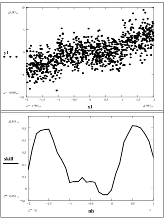
Figure 1: Importance of assessing the skill of the model from the predictor space.

Realizations shown in Figure1a (top) are generated with the predictand y depending on two predictors, x1 and x2 with x1 influencing the predictand only if the absolute value of the

predictor is greater than the threshold value of 1. The underlying model is yt = 2x1t+0.5x2t +εt if |x1t| > 1 and yt = 0.25x2t +εt if |x1t| ≤|1. The noise term εt follows i.i.d with Normal distribution having zero mean and a standard deviation of 2. The predictors follow uniform distribution between -2 to 2. A total of n= 1000 realization is generated from this model. This could be analogously compared to two predictors with anomalous SSTs influencing the local

hydroclimatology and the predictor x1 primarily enforces teleconnection such as ENSO and predictor x2 is the local SSTs influencing the streamflow. The correlation between y and x1 is 0.671 and y and x2 is 0.134. Thus, this would enforce one to give higher importance to predictor x1. Figure 1b shows the correlation between the predictand y and the predictor x1 by considering a moving on x1 with a bandwidth of 1. The plot gives the correlation between y and x1 against the lower bound of the bandwidth of the moving window on x1. Thus, the skill for nh= - 2 denotes the correlation between y and x1 evaluated for the set of x1 values between -2 to -1. Note the clearly insignificant relationship between y and x1 during nh = -1 to 0. Thus, by evaluating the model from the predictor state space, the approach evaluates the performance of alternate models that includes climatological ensembles as well.

2 1.5 1 0.5 0 0.5 1 1.5 2

10 5 0 5 10 9.387

8.608

−

y1

1.993 1.994

− _x1

2 1.5 1 0.5 0 0.5 1

0.1 0 0.1 0.2 0.3 0.4 0.5 0.519

0.053

−

skill

1 2

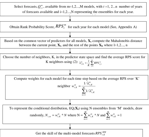
Figure 2: Flowchart of the multi-model ensembling algorithm described in Section 3.2 for fixed number of neighbors ‘K’ in evaluating the model skill from the predictor state space. To apply the same algorithm for kt that gives the minimum RPS from the multimodel ensembles, compute

MM k t

RPS _, for k= 1,2,..., n-1 and choose k that corresponds to minimum RPS_tMM_,k . Thus, by computing RPS_tMM_,k for all the data points, we choose the number of neighbors, kt, that has the minimumRPS_tMM_,k .

Select forecasts,Q_im_,t, available from m=1,2...,M models, with t =1, 2...n number of years of forecasts available and i=1,2...,N representing the ensembles for each year. k represents models.

Obtain Rank Probability Score,

RPS

Based on the common vector of predictors for all models, X, compute the Mahalonobis distance between the current point, Xt, and the rest of the points Xl, where l=1,2..., n

Choose the number of neighbors, K, in the predictor state space and find the average RPS score for K neighbors using (2):

_∑

= = λ K j m j RPS K 1 ) ( m K t, 1

Compute weights for each model for each time step based on the average RPS over ‘K’ neighbor

∑

To represent the conditional distribution, f(Qt|Xt) using N ensembles from ‘M’ models, draw

randomly, * whereN * and 1

1 , 1 , , , = =

∑

∑

t w N w N w

N

0 200 400 600 800 1000 1200 1400 1600 1800 2000 J a n F e b M a r A p r M a y J u n e J u ly A u g S e p O c t N o v D e c Months S tr e a m fl o w (f t 3 /s ) average 25th percentile 75th percentile

Low Flow Season JAS - 14% High flow season

JFM - 46%

(a) 53 20 8 ₆ 4 0 10 20 30 40 50 60

0 1 2 3 4 5 6

Principal component (PC) i

% v a ri a n c e e x p la in e d (c)

Figure 3: Hydroclimatology of Neuse Basin: (3a) Seasonality of Neuse Basin (3b) Climatic Predictors that influence the streamflow (3c) Scree Plot and the variance of the principal components. Top figure shows the seasonality of Neuse basin with the flow during JAS accounting for 14% of the annual streamflow. Insert in figure 3(a) show the location of Neuse basin in NC. Figure 3(b) shows the correlation between SSTs in the Pacific and Atlantic oceans and the observed streamflows into the Falls Lake. The correlations that are significant at 95% (±0.23) are only shown. Figure (3c) shows the scree plot for the principal components of the observed SSTs and their % explained variance. The dominant zone of predictability for each PC is also indicated.

0 200 400 600 800 1000 1200 1400 1600 1800 2000

1988 1990 1992 1994 1996 1998 2000 2002

Year F lo w s ( ft 3 /s ) Observed Conditional mean 25th percentile 75th percentile 0.55 Predicted) (Observed, ρ = ∧ (a) 0 200 400 600 800 1000 1200 1400 1600 1800 2000

1988 1990 1992 1994 1996 1998 2000 2002

Figure 5: Performance of individual models from predictor state space by considering K=10 neighbors. (5a) Correlation Vs PC1. (5b) RPS Vs PC1. (5c) Correlation of regression Vs

Correlation of resampling (5d) RPS of regression Vs RPS of resampling. RPS is computed from the leave-1-out cross validated forecasts shown in Table 2 for individual models by assuming K=10 in equation (2). Correlation is computed between the observed and ensemble mean of the leave 1 out forecasts in Table 2 by considering 10 neighbors in the predictor state space. Note the consistent poor performance of both the models in Figure 5(c) as well as for high negative values of PC1. -1 -0.5 0 0.5 1

-1 -0.5 0 0.5 1

Correlation(resampling) C o rr e la ti o n (r e g re s s io n

) _{Resampling poor}

Regression poor Both good Both poor (c) 0 0.2 0.4 0.6 0.8 1

0 0.2 0.4 0.6 0.8 1

RPS(resampling) R P S (r e g re s s io n

) Regression poor

Resampling poor (d) 0 0.2 0.4 0.6 0.8 1

-10 -8 -6 -4 -2 0 2 4 6

PC 1 R P S resampling regression (b) -1 -0.8 -0.6 -0.4 -0.2 0 0.2 0.4 0.6 0.8 1

-10 -8 -6 -4 -2 0 2 4 6

0 200 400 600 800 1000 1200 1400 1600 1800 2000

1988 1990 1992 1994 1996 1998 2000 2002 Year F lo w s ( ft 3 /s ) Observed Conditional mean 25th percentile 75th percentile 0 200 400 600 800 1000 1200 1400 1600 1800 2000

1988 1990 1992 1994 1996 1998 2000 2002 Year F lo w s ( ft 3 /s ) Observed Conditional mean 25th percentile 75th percentile

0 10 20 30 40 50 60 70 80

-15 -10 -5 0 5 10

PC1

N

e

ig

h

b

o

rs

,K

0 0.1 0.2 0.3 0.4 0.5 0.6 0.7 0.8

0 0.1 0.2 0.3 0.4 0.5 0.6 0.7 0.8

Forecast probability O b s e rv e d r e la ti v e f re q u e n c y

Perfect Reliability Resampling Regression Multi model

(a)

Perfe ct Re

liabil ity

Total deviation from perfect reliability Err(Resampling)=0.26 Err(regression)=2.17 Err(Multi-model)=0.22 0 0.1 0.2 0.3 0.4 0.5 0.6 0.7

0 0.1 0.2 0.3 0.4 0.5 0.6 0.7

Forecast probability O b s e rv e d r e la ti v e f re q u e n c y

Perfect Reliability Resampling Regression Multi model

Perfe ct Re

liabil ity

Total deviation from perfect reliability Err(Resampling)=0.70

Err(regression)=1.41 Err(Multi-model)=0.19

(b)