Combining Gene Expression and Molecular Marker Information for Mapping
Complex Trait Genes: A Simulation Study
Miguel Pe´rez-Enciso,*
,1Miguel A. Toro,
†Michel Tenenhaus
‡and Daniel Gianola
§*Station d’Ame´lioration Ge´ne´tique des Animaux, INRA, BP 27, 31326 Castanet-Tolosan, France,†Departamento de Mejora Gene´tica Animal, INIA, 28040 Madrid, Spain,‡HEC School of Management, 78352 Jouy-en-Josas, France and§Department of Animal Sciences,
University of Wisconsin, Madison, Wisconsin 53706
Manuscript received January 6, 2003 Accepted for publication April 4, 2003
ABSTRACT
A method for mapping complex trait genes using cDNA microarray and molecular marker data jointly is presented and illustrated via simulation. We introduce a novel approach for simulating phenotypes and genotypes conditionally on real, publicly available, microarray data. The model assumes an underlying continuous latent variable (liability) related to some measured cDNA expression levels. Partial least-squares logistic regression is used to estimate the liability under several scenarios where the level of gene interaction, the gene effect, and the number of cDNA levels affecting liability are varied. The results suggest that: (1) the usefulness of microarray data for gene mapping increases when both the number of cDNA levels in the underlying liability and the QTL effect decrease and when genes are coexpressed; (2) the correlation between estimated and true liability is large, at least under our simulation settings; (3) it is unlikely that cDNA clones identified as significant with partial least squares (or with some other technique) are the true responsible cDNAs, especially as the number of clones in the liability increases; (4) the number of putatively significant cDNA levels increases critically if cDNAs are coexpressed in a cluster (however, the proportion of true causal cDNAs within the significant ones is similar to that in a no-coexpression scenario); and (5) data reduction is needed to smooth out the variability encountered in expression levels when these are analyzed individually.
A
powerful tool for monitoring gene expression in as phenotypes and analyzed one by one separately,i.e., treated as any quantitative trait in a usual QTL analysis parallel is cDNA microarray technology. Atpres-ent, microarrays are being used for improving our (Bremet al. 2002;Schadtet al.2003). This approach encounters several difficulties, such as the problem of knowledge about disease classification as well as for
un-assigning correct significance levels when multiple statis-raveling complex genetic regulation networks (
Knud-tical tests are conducted or the presence of skewed
distri-sen 2002). So far, massive expression data have been
bution of gene expression measurements. In addition, mostly utilizedper se, without regard to marker
informa-many genes are regulated and expressed in concerted tion. However, combining both sources of information
action (Caron et al. 2001), so a gene-by-gene analysis may yield a more accurate picture of genetic processes
may not be insightful enough. Further, a huge number underlying complex traits than that currently obtained
of simultaneous QTL analyses would be hard to inter-by using them separately. For example, expression data
pret biologically. can perhaps be used to improve estimates of location
An arguably more powerful and appealing approach of genes affecting complex traits or quantitative trait loci
may consist of detecting some underlying pattern of (QTL). Seemingly, this issue has not been addressed,
expression that is correlated with the trait of interest. although it has been suggested (JansenandNap2001)
This implies that some sort of data reduction would be that genomics and genetics should be merged into
“ge-needed. Techniques for this purpose include,e.g., prin-netical genomics.” This field would involve expression
cipal components, canonical analysis, and partial least profiling, marker genotyping, and the statistical tools
squares (PLS). Principal components, a widely used tech-that have been developed for QTL analysis.
nique in multivariate analysis, has been already applied There are several potentially useful alternatives to
to expression data (Alter et al. 2000; Holter et al.
combining microarray and marker data. For instance,
2000, 2001;Westet al.2001). PLS, on the other hand, one may study the genetic basis of the individual
expres-may be viewed as a compromise between multivariate sion levels themselves;Eaveset al.(2002) gives an
illus-regression and principal component analysis (
Tenen-tration. In this setting, expression levels are regarded
haus1998;Hastieet al.2001). The objective here is to find some linear combination of the original expression measurements, or “supergene,” that maximizes the cor-1Corresponding author:SAGA-INRA, BP 27, 31326 Castanet-Tolosan,
France. E-mail: [email protected] relation with some response variable of interest, such
MATERIALS AND METHODS as the phenotype for a disease trait. In PLS, each new
supergene is obtained such that it is orthogonal to all Underlying genetic model:It is assumed that the probability previously defined supergenes (Tenenhaus1998;Ngu- that a disease affects an individual depends on the value of
some latent, unobservable, variable (often referred to as
liabil-yenandRocke2002). In PLS, all variables (gene
expres-ity). The relationship between the probability of disease and sion levels and phenotypes) are used to arrive at the
liability may not be linear. We express liability as some un-supergenes, whereas only the expression measurements
known linear combination of gene expression levels. Consider-are used in principal component regression. Enlight- ing a single QTL affecting the disease, the allelic variants at ening comparisons of PLS, principal component regres- the QTL are assumed to produce a shift in mean liability, thus sion, and ridge regression have been published (Frank affecting the risk of individuals carrying a given mutation. Note that the effect of the gene is mediated through the andFriedman1993).
relevant expression levels;i.e., its impact on the probability of If some pattern of expression correlated with the trait
an individual contracting the disease is indirect. of interest can be identified, the microarray data could
Simulation strategy:Current knowledge about possible sta-be used to refine our knowledge about the genetic basis tistical distribution(s) followed by gene expression levels mea-of a complex trait (e.g., a disease), instead of being viewed sured with microarray technology is scant. Further, it has been noted that expression levels may be intercorrelated in a com-merely as an additional set of phenotypes to be analyzed
plex manner, which would require posing some multivariate as any other quantitative trait. For instance, expression
distribution. Hence, a standard simulation of expression levels data could be used to improve QTL mapping if the
would be probably unrealistic, at least given present knowl-following two conditions were met: (1) some of the gene edge. To circumvent this problem here we propose, instead, expression levels must be under (at least partial) genetic to use available real data and simulate the underlying liability
conditionallyon observed expression levels contained in real control of the QTL and (2) some of these heritable
data, thus reducing dramatically the arbitrariness in the simu-gene expression levels must be related to the disease.
lation. Suppose the “true” liability of theith individual ishi⫽
Otherwise, accommodating expression data in a statisti- ⬘
xi, whereis a vector of unknown weights given to each
cal model would reduce the power of tests (due to an of the gene expression levels, with the latter contained in additional, unneeded, level of parameterization) and vectorxi. It is reasonable to suppose that most of the values increase experimental costs. There is evidence that both inwould be zero because the majority of the genes will not affect the trait of interest. Assume now that probability of conditions can be met, at least in some situations. For
disease is related to liability via a logistic function, so that the instance, p53 mutations lead to a differential gene
ex-chance of individualibeing affected (yi⫽1) is given byP(yi⫽
pression in breast cancer-affected and -unaffected indi- 1|
hi) ⫽ exp(hi)/[1⫹ exp(hi)]. Hence, given hi, the disease
viduals (Sorlieet al.2001). Likewise, the levels of heat- status for each individual can be simulated using a Bernoulli shock protein differ between congenic strains in rats, distribution with probabilityP(yi⫽1|hi). The logistic
transfor-mation was chosen because it is widely used for modeling and which suggests a genetic basis for the observed
differ-analyzing binary data (HosmerandLemeshow2000). ence in expression (Dumaset al.2000).
Different plausible scenarios of gene interaction models Large-scale experiments involving both microarray
were considered to generate weights. First, we allowed gene and marker genotyping are not foreseeable in the imme- expression levels included in the liability to be independent diate future. Rather, we envisage trials where a relatively or not. In the first case (referred to as “diffuse”), the cDNA clones having an effect on liability were selected indepen-small number of individuals, say⬍100, have their gene
dently and with equal probability within those whose expres-expression levels monitored as well as genotyped for
mo-sion level had been measured in the microarray. In the second lecular markers; there may be additional individuals
case (“clustered”) the first cDNA clone was chosen randomly, whose genotypes are known but are not microarrayed. and the rest were selected with a probability that was propor-Two of the most promising experimental approaches in- tional to the absolute value of the correlation of expression volve recombinant inbred lines and association studies, levels between the first cDNA and the other candidates. We generated weights using either a uniform (0, 1) distribution where controls and cases are carefully stratified to avoid
or an exponential distribution with mean ⫽ variance ⫽ 1. confounding effects. Use of recombinant lines is possible
Signs (⫹/⫺) of the weights were selected at random in the only with laboratory species (Eaveset al.2002), whereas diffuse case and had the same sign as the correlation in the case/control studies constitute one of the most typical clustered case. cDNAs that were not selected received a weight research protocols in humans. Although we concentrate of zero. Thus, there was a total of four hypothetical scenarios for eliciting the true weight vector: diffuse/uniform (D/U), on case/control designs, the principles outlined in this
diffuse/exponential (D/E), clustered/uniform (C/U), and work apply to other statistical methods and/or designs.
clustered/exponential (C/E). The four scenarios are briefly Our objective is to study the issue of whether or not
described in Table 1. Note that the variance of liabilities cDNA microarray data can be used to refine genomic changes according to the scenario and the number of expres-position estimates of genes that affect a complex trait, sion levels in the liability.
In all scenarios, the set of weights was such that the such as a disease. The impact of the gene expression
in-frequency of affected individuals,P(y⫽1), in the whole popu-formation is quantified under a range of plausible
ge-lation was bounded between 45 and 55%. This condition stems netic architectures, including presence or absence of
TABLE 1
Gene expression scenarios considered
Scenario Description 2
h a
Diffuse/uniform (D/U) Clones inhchosen at random,bweights sampled from 1.8, 5.5, 8.5, 17.8
uniform (0, 1)
Diffuse/exponential (D/E) Clones inhchosen at random, weights sampled from 6.5, 19.3, 49.0, 92.9 exponential ⫽1
Clustered/uniform (C/U) Clones inhchosen proportional to correlation, weights —,c8.9, 17.2, 39.9
sampled from uniform (0, 1)
Clustered/exponential (C/E) Clones inhchosen proportional to correlation, weights —,c26.8, 56.9, 168.7
sampled from exponential ⫽1
aVariance of true liabilities averaged over replicates when 1, 5, 10, and 20 genes are included in the liability, respectively.
Disease incidence was 50% in all scenarios.
bUnderlying true liability.
cSame as without clustering.
draws of weights were required because a 50% incidence is and a position at ␦ morgans is 1 ⫺ exp(⫺␦), where is the number of generations since the mutation (McPeekand simply ensured when the average of the weights is close to
zero. Weights were scaled using the standard deviation of each Strahs1999). For those haplotypes not carrying the mutation, the SNP alleles were sampled assuming linkage equilibrium cDNA level.
We further assumed a biallelic additive QTL, where a mu- between markers. We used a frequency of 0.7 for the most common allele for all SNPs, and we set ⫽ 500. The QTL tant allele shifts the mean of the underlying susceptibility.
Individuals carrying this allele are more prone to contracting was in position 0.
With respect to the expression data, a breast cancer data the disease, but this relationship is not perfect (incomplete
penetrance). In the context of our model, this means that the set (Sorlieet al.2001) was used; at the time it was one of the largest data sets publicly available at the Stanford microarray mutation may affect several cDNA levels to a different extent,
depending on the values of the elements of the vector. It public database (http://genome-www5.stanford.edu/microarray/ was assumed that the distribution of the liabilities given the SMD/). It consists of 85 samples and the expression levels of genotype (g) could be approximated by a normal distribution 456 cDNA clones, what the authors called the “intrinsic data
f(h|g)⫽N(g,2); the standardized QTL additive effect was set” (Perouet al.2000). The data reported are the log2 ratios
defined asa⫽(g⫽AA⫺ g⫽BB)/2, withAandBdenoting the between the mean intensities of the test sample and of a
two QTL alleles. Givenh, the probability of an individual i control sample that consisted of a pool of tissues. The log having genotypekis, applying Bayes’ theorem, transformations were used to make distributions more “nor-mal,” and the base 2 is convenient because it makes
interpreta-P(gk|hi)⫽P(gk)f(hi|gk)/
兺
3
j⫽1
P(gj)f(hi|gj), (1) tion easier. Full details of the experimental and statistical
protocols are available online at the web page cited above. Only the 71 cDNAs that did not have any missing record were where P(gk) is the frequency of genotypek, k ⫽1, 2, 3 for
eligible to enter into the true liability. Thus, a numberngof
the biallelic QTL. Equation 1 allows us to assign a genotype
cDNA levels was chosen at random out of the 71, and the probability to anith individual, given its observed microarray
weightswere adjusted as specified above for each of theng
data, the weights, the genotype frequenciesP(g), and the
expression levels. The values of number of genes studied were parameters of the normal distribution. However, one needs
ng⫽1, 5, 10, or 20. The QTL effects werea⫽0.5, 1, and 1.5
to specifygand2. The mean of the distribution follows
di-SD units. The QTL genotype frequenciesP(g) were chosen rectly from the desired standardized QTL effect,a. The
vari-to represent two extreme distributions, 0.25/0.50/0.25 and ance of the liabilities is the variance of a mixture and can be
0.5/0.0/0.5 for theAA/AB/BBgenotypes, respectively. The written as Var(h)⫽Eg[Var(h|g)] ⫹ Varg[E(h|g)]. Given a
stan-latter frequencies correspond to a case/control study where dardized genotypic effect,a⫽(g⫽AA⫺ g⫽BB)/2, we solved
the disease allele is recessive and at very low frequency; in this for2using an iterative algorithm such that Var(h) was equal
case, all affected individuals are homozygous and the fre-to the observed variance of the liabilities in our sample.
quency of heterozygous individuals in the normal population Once an individual’s genotype was obtained, the rest of
is negligible. Five hundred simulation replicates were carried the haplotype was simulated. Ten biallelic markers
[single-out for each scenario. In each replicate a new set ofngcausal
nucleotide polymorphisms (SNPs)] were generated every
cDNAs was chosen, and new values for, QTL genotypes, 0.5 cM, following a simple model for linkage disequilibrium
phenotypes, and haplotypes were simulated, always condition-decay. Briefly, a founder haplotype was chosen, sampling a
ally onSorlieet al.’s (2001) data. combination of SNP alleles at random. This was assumed to
Figure 1 summarizes the main steps in the simulation. First, be the original haplotype where the QTL mutation occurred.
a series of weightsare chosen according to any of the four Then, for individuals that had one or two mutant QTL alleles,
scenarios described (Table 1), and the individual liabilities one or two haplotypes carrying the mutation were simulated.
are obtained; the obtained liability population is a mixture, As generations proceed, the probability that at least one
re-wherefrom the QTL genotypes are sampled using Equation combination occurs within the 0.5-cM region surrounding the
1 for each individual; the haplotypes are obtained; and pheno-QTL will increase and thus the homology with the founder
types are sampled from binomial processes depending on haplotype will disappear gradually. The length of the
nonre-individualhvalues. combinant region starting from the QTL was sampled,
Figure 1.—Simulation scheme. (1) Choose weights assigned to cDNA clones for obtaining individual liabilities, after fixing a number of cDNA clones and the gene expression scenario; (2) sim-ulate binary phenotypes from the liability using the logistic distribution; (3) simulate QTL types given liability, QTL effect, and QTL geno-type frequencies using Equation 1; and (4) simu-late haplotypes from QTL genotype, marker allele frequencies, and number of generations since mutation.
was carried out at the “true” position of the QTL using either 2, . . . ,qandi⫽1, 2, . . . ,n. The goal of PLS logistic regression is to find a linear combination of the expression levels for the phenotypic information only or the phenotypes and the
microarray data. An analysis of variance (ANOVA) was used modeling to test differences in phenotype (y) or estimated liability (hˆ)
amongAA,AB, andBBgenotypes. The liability for individual
P(yi⫽1)⫽exp
冤
兺
k⫽1
(w⬘kxi)bk
冥
冒
冦
1⫹exp冤
兺
k⫽1
(w⬘kxi)bk
冥冧
iwas estimated ashˆi⫽兺k⫽1bktik, withbandtobtained by
lo-gistic PLS regression as explained below, and whereis the
number of components fitted. Subsequently, an ANOVA was ⫽exp(hi)/[1⫹exp(hi)], performed at each of the 10 SNPs using the marker genotype
whereis the number of PLS components,wkis aq
-dimen-as cl-dimen-assification factor. The difference betweenPvalues of the
sional vector containing the weights given to each original ANOVAF-tests using either the phenotype or the estimated
variable in thekth component (defining a “supergene”),xiis
liability provides an indication of the relative power of the
the vector containing theqexpression levels for individuali, different sources of information for locating a QTL. The PLS
bkis the regression coefficient of the underlying variable on
analysis was done with all 456 expression levels, rather than
thekth component variable, andhis the underlying liability. with only the 71 with no missing data.
The elements ofwandbcan be obtained as follows (Esposito -Suppose that the matrixX⫽{xij} contains the expression
1. For each variablej⫽1, 2, . . . ,qcompute its significance in a logistic regression, each variable in turn using the modelP(yi⫽1)⫽exp(b0⫹ 1jxij)/[1⫹exp(b0⫹ 1jxij)].
2. Select those variables that are significant; The first super-gene is defined, for eachith individual, ast1i⫽w⬘1xi, with
w1j⫽ 1j/√兺j僆ᑬ121j, where the sum ofjis over the significant
cDNAs. An extremely useful property of this approach is that it can deal with missing data in the regressors xij, a
common phenomenon with microarray data. Suppose a subset ofxijare actually measured in theith individual, the
weights are given by1j/√兺j僆ᑬ1*21j, whereᑬ1* is the subset of
significant variables present for that individual, and the superscript 1 indicates the significant subset in the first PLS component.
3. The regression coefficientb1is obtained from fittingP(yi⫽
1)⫽exp(b0⫹b1t1i)/[1⫹exp(b0⫹b1t1i)].
4. The next PLS component is obtained by testing again each of the original q variables plus the previous surpergene
P(y ⫽ 1)⫽ exp(b0 ⫹ b1t1⫹ 2jxj)/[1⫹ exp(b0 ⫹ b1t1⫹ 2jxj)], j ⫽ 1, 2, . . . , q. Once the new set of significant
variables is determined, the second supergene is obtained fromt2i⫽w⬘2xi, withw2j⫽ 2j/√兺j僆ᑬ222j, applying identical
considerations as before with missing observations.
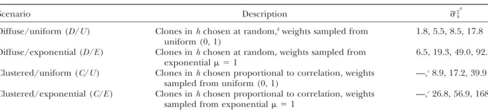
Figure2.—(a) Percentage of cDNA clones that do influ-This process is repeated until no new variable (expression ence true liability found to be significant (and included in level) is found to be significant. It should be noted that a any of the PLS components) as a function of the number of given gene expression level may be significant in only one clones that affect underlying liability and according to the PLS component, whereas others may be significant in more gene expression scenario. (b) Number of cDNA clones in the than one component. Moreover, it is also possible (actually, PLS component, as a function of the number of clones that this is often the case) that a variable is not significant in com- affect underlying liability and according to the gene expres-ponentkbut significant in componentk⫹1. Thus, it is wise sion scenario. The results are the average over 500 simulation not to discard a set of variables fully from the first component. replicates and across QTL frequencies and effects, which were In this study, a variable was declared significant if its estimate very similar. Inset: D/U, diffuse/uniform scenario; D/E, dif-divided by its standard deviation, which is approximately nor- fuse/exponential; C/U, cluster/uniform; C/E, cluster/expo-mally distributed, was⬎3.27, a two-tailed 0.1% significance nential (Table 1). Note that a cluster scenario is not defined level. Logistic coefficients can be estimated using a variety for a single clone.
of algorithms and software. Here we employed the publicly available subroutines of A. Miller (http://users.bigpond.net. au/amiller/).
implemented in some commercial packages (Umetrics
2001). Nevertheless, the problem caused by multiple tests cannot be overemphasized. Here, we used a rather RESULTS AND DISCUSSION
high significance level because the number of clones One of the main issues arising when microarray data was relatively small but more stringent levels should be are analyzed is the “excess” of potential regressors rela- used in larger data sets. The false discovery rate can be tive to the much smaller number of individuals arrayed. a useful alternative to the usual Bonferroni corrections Here, we have proposed to combine linearly a set of ex- employed with multiple testing (Storeyand
Tibshir-pression levels instead of studying each cDNA clone ani 2003). Frank and Friedman (1993) have shown separately. Among the many available techniques in how PLS, principal component regression, and ridge multivariate analysis, we have chosen the partial least- regression can be interpreted in terms of applying a squares approach (Woldet al.1983). This technique is penalty on the usual least-squares estimates;i.e., these quite popular in chemometrics but much less so in are shrinkage estimators. It has been recently discussed genetics. The main advantages of PLS lie in its simplicity (Gianolaet al.2003) how classical shrinkage estimators (it can be implemented using standard statistical tools); can be superseded by Bayesian counterparts for marker-its versatility (e.g., generalized linear models can be fit- assisted selection. We are not aware of the existence of ted, as in the present study); and in the fact that the any equivalent of PLS in the Bayesian context; this could components are derived using both the regressors (X) be an interesting area of research either by itself or and the dependent variable, the latter being disease in how it relates to microarray analysis. Nonetheless, a status here. Tests of hypotheses are carried out using drawback of most of the dimension-reducing tech-standard techniques. We used Wald’s test to ascertain niques, PLS included, is that the results are usually diffi-whether a given expression level was significant but cult to interpret biologically.
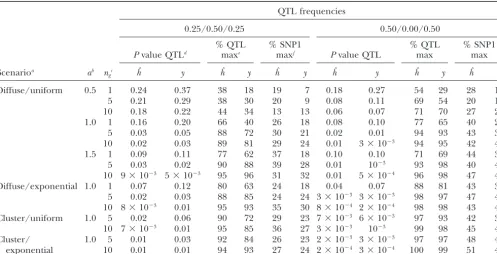
Figure 3.—Effect of the gene expression scenario on correlations (r) between true liability and different variables (plain lines): esti-mated liability (light gray, labeled hh_hat), estimated liability when deleting the cDNA clones that affect true liability from the data set (dark gray, labeled hh_hat*), and phenotype (black, la-beled hy). Correlations be-tween genotypic value and different variables (starred lines) are true liability (dashed black lines, labeled gh), estimated liability (solid light gray, labeled gh_hat), estimated liability when the genes affecting true liability are removed (solid dark gray, labeled gh_hat*), and phenotype (solid black, la-beled gy). Results corre-spond to QTL effect⫽1 SD and QTL frequencies 0.25/ 0.50/0.25, averaged over 500 simulation replicates.
the actual causal genes. A main issue, then, is to evaluate -negative breast cancers (Gruvbergeret al.2001;Khan
et al.2001;Westet al.2001;Pe´rez-Encisoand
Tenen-the chance of identifying a gene whose expression
af-fects liability. Figure 2a shows that this depends mostly haus2003).
A positive association was found between the number on the number of cDNA clones actually involved inh;
we did not find any influence of the QTL effect or of of cDNA clones inhand the number of clones included inhˆ(Figure 2b), and the association was even stronger the QTL allele frequencies, so results were averaged
over effects and frequencies. If liability is monogenic, when causal cDNAs were coexpressed in a cluster. How-ever, as the number of clones inhincreased, the relative the probability that the cDNA clone is included in at
least one of the PLS components (supergenes) varies effect of each clone is expected to decrease, especially in a diffuse scenario, and so does the power of PLS for between 60%, when weights are uniformly distributed,
and 80%, when an exponential distribution is used. This identifying each effect. This may explain the lack of linearity of the association in the diffuse scenario. The simply reflects the fact that weights are, on average,
larger in the exponential than in the uniform scenario. number of PLS components fitted was also affected by the actual number of cDNA clones in the liability: only The distribution of weights did not seem to affect the
results appreciably when liability was polygenic. Never- one PLS component was retained inⵑ95% of replicates when the true liability was monogenic (ng ⫽ 1). This theless, clustering of gene effects increased the number
of true significant cDNAs identified. This is a conse- does not mean that the PLS component consisted of a single cDNA, as the number of genes in the PLS compo-quence of a higher number of total significant cDNAs
in PLS in clustered compared to diffuse scenarios (Fig- nent was ⵑ4 (Figure 2b). A second component was significant when liability was polygenic in 10–20% of ure 2b). In fact, the percentage of true causal cDNAs
among significant ones was similar in diffuse and in replicates. An exponential distribution for the weights increased the percentage with two PLS components clustered scenarios. There is clear evidence that
coex-pression can be strong in both humans and Drosophila fitted, but this percentage was roughly the same for 5, 10, or 20 genes within this scenario. This may reflect (Caronet al. 2001;Arbeitman et al. 2002). All in all,
on average, only between two and four real causal clones the fact that PLS is computed such that the number of components is minimized.
are identified as significant when 20 expression levels
are actually involved in the liability (see Figure 2a). This The results shown in Figure 2a do not imply that the liability was estimated poorly. On the contrary, the may explain why discordant sets of cDNA clones are
TABLE 2
Main results
QTL frequencies
0.25/0.50/0.25 0.50/0.00/0.50
% QTL % SNP1 % QTL % SNP1
Pvalue QTLd maxe maxf Pvalue QTL max max
Scenarioa ab n
gc hˆ y hˆ y hˆ y hˆ y hˆ y hˆ y
Diffuse/uniform 0.5 1 0.24 0.37 38 18 19 7 0.18 0.27 54 29 28 18
5 0.21 0.29 38 30 20 9 0.08 0.11 69 54 20 14
10 0.18 0.22 44 34 13 13 0.06 0.07 71 70 27 24
1.0 1 0.16 0.20 66 40 26 18 0.08 0.10 77 65 40 20
5 0.03 0.05 88 72 30 21 0.02 0.01 94 93 43 37
10 0.02 0.03 89 81 29 24 0.01 3⫻10⫺3 94 95 42 42
1.5 1 0.09 0.11 77 62 37 18 0.10 0.10 71 69 44 30
5 0.03 0.02 90 88 39 28 0.01 10⫺3 93 98 40 42
10 9⫻10⫺3 5⫻10⫺3 95 96 31 32 0.01 5⫻10⫺4 96 98 47 47
Diffuse/exponential 1.0 1 0.07 0.12 80 63 24 18 0.04 0.07 88 81 43 38
5 0.02 0.03 88 85 24 24 3⫻10⫺3 3⫻10⫺3 98 97 47 47
10 8⫻10⫺3 0.01 95 93 35 30 8⫻10⫺4 2⫻10⫺4 98 98 43 43
Cluster/uniform 1.0 5 0.02 0.06 90 72 29 23 7⫻10⫺3 6⫻10⫺3 97 93 42 35
10 7⫻10⫺3 0.01 95 85 36 27 3⫻10⫺3 10⫺3 99 98 45 41
Cluster/ 1.0 5 0.01 0.03 92 84 26 23 2⫻10⫺3 3⫻10⫺3 97 97 48 47
exponential 10 0.01 0.01 94 93 27 24 2⫻10⫺4 3⫻10⫺4 100 99 51 47
aSee Table 1 for description of each scenario.
bQTL effect in SD units.
cNumber of cDNA levels in true liability.
dMean ANOVAPvalue using estimated liability (hˆ) or phenotype (y).
ePercentage of replicates when maximum statistics, using estimated liability (hˆ) or phenotype (y), coincided with QTL position. fPercentage of replicates when maximum statistics, using estimated liability (hˆ) or phenotype (y), coincided with closest SNP
when QTL genotype was not included in the region scan.
Figure 3, where the correlation between true and esti- the phenotype when liability is polygenic. A clustered scenario makes the loss in accuracy smaller when causal mated liability is labeled “hh_hat” (the plain light gray
line). This correlation was independent of the QTL cDNAs are not spotted. Figure 3 also depicts the correla-tions between genotypic values and liability, its estimate, effect (results not shown), but it increased slightly as
the number of cDNAs in the true liability increased. or the phenotype (starred lines). The dashed black line, labeled “gh” (correlation between genotype and true Figure 3 also shows that the advantage of using
microar-ray data over simply the phenotypes was inversely related liability) sets the maximum correlation that can be ex-pected. The trends of correlations with true liability or to the number of cDNAs in the true liability and that
it was maximum when liability was monogenic (compare genotype were similar (compare plain and starred lines). Again, as the number of cDNAs in liability increased, the lines labeled hh_hatvs.“hy”). Interestingly, a
clus-tered scenario was more favorable than a diffuse sce- the value of phenotypic information relative to that of estimated liability increased. Clustering, instead, favored nario, especially when weights were uniformly
distrib-uted. the usefulness of the estimated liability.
Table 2 presents the ANOVAPvalues obtained using An implicit assumption of our model is that the clones
that influence liability have been spotted in the microar- eitherhˆor phenotype (y), as well as the percentage of replicates where the significance was maximum at the ray. If this were not so, the possible advantage of using
microarray data would be reduced, although it would QTL position or at the closest SNP (SNP1) when the QTL position was not included in the genome region seldom be nil because of possible correlations of
expres-sion between spotted and nonspotted genes. We evalu- scan. These percentages somewhat reflect the confi-dence that we can have in the estimated QTL position ated this possibility by removing from the data set all
cDNA clone data involved inhand carrying out the PLS with and without microarray information. Not all cases analyzed are reported to facilitate legibility. First, note analysis subsequently. It can be seen (Figure 3, dark gray
Figure4.—Example of profile of thePvalues: ANOVAP
value with estimated liability (—) and ANOVA Pvalue with phenotype (- - -). Cluster/uniform scenario with QTL effect⫽ 1 SD, five cDNA clones in true liability, and QTL frequencies equal to 0.25/0.50/0.25, averaged over 500 simulation repli-cates, is shown.
frequencies. Other things being equal, microarray data will be more useful if liability is monogenic, as could
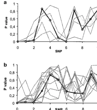
Figure5.—P-value profile of a single replicate, for the esti-be expected from results in Figure 3. Similarly, the
per-mated liability (thick circled line) and each of its individual centage of replicates where the position of maximum cDNA components (thin gray lines), QTL effect ⫽1 SD in significance coincided with the QTL position was com- the diffuse/uniform scenario. (a) The true number of cDNA paratively better withhˆthan withyat small QTL effects. clones in the liability is 1; (b) the number of cDNA clones is
10. The QTL is in position 0. Clustering and an exponential scenario favored using
hˆ over only the phenotype when significance was low. Figure 4 displays an illustration of the performance
when all expression levels are analyzed separately; recall of the test over the interval considered when we use the
that a typical microarray experiment consists of thou-phenotypey(dashed line) or the estimated liability with
sands of measurements. This means that it may be very PLShˆ(solid line). On average, the point of maximum
difficult to interpret all sets of QTL profiles when cDNA significance (minimumPvalue) coincides with the QTL
levels are analyzed individually. position (position zero), and over the entire interval the
The four scenarios considered in this work are ideal-power is larger when using microarray data than when
ized representations of a variety of possible gene interac-using the disease status (phenotype) only. Although the
tion networks. The diffuse/uniform case corresponds to average test was maximum at the QTL position, see
Ta-the simplest scenario and may be viewed as a “null hy-ble 2 for the percentage of replicates when this actually
pothesis” model. In the diffuse/exponential model we happened. Association studies are well known for the
study the effect of unequal gene contributions, which difficulty in obtaining replicable results (Emahazionet
is perhaps a more realistic assumption. Overall, it seems
al.2001), which is due, in part, to the wide variability
that gene clustering is far more relevant than the fact that disequilibrium exhibits (Nordborg and Tavare´
of having unequal weights (e.g., Figures 2 and 3). There 2002). Note that when the causal (QTL) mutation was
is ample evidence of coexpression of large clusters of not genotyped, the closest SNP coincided with the
maxi-genes (Caronet al.2001;Arbeitmanet al.2002), but in mum statistic in⬍50% of the replicates for most of the
the context of this work we are interested in coexpressed cases studied (Table 2).
genes that are causal as well. If coexpressed genes are The purpose of this article was not to assess extensively
not causal, the number of genes in the PLS components the impact of disequilibrium variability on cDNA-QTL
will increase (Figure 2a), but not the number of causal studies. However, the study illustrates that a
PLS-esti-significant genes. mated liability will normally have a more stable behavior
There is, thus far, no empirical evidence about the than any of its components (i.e., cDNA measurements
genetic basis of gene expression on a genome-wide scale here) taken individually. For instance, Figure 5 displays
in outbred populations, although some experiments con-results for two individual replicates in the
diffuse/uni-cerning QTL analysis in crosses between inbred stocks form scenario where the estimated liability and all of
have begun to appear, notably that ofBremet al.(2002) its individual components are shown when the true
lia-in yeast but also lia-in mice and maize (Schadtet al.2003). bility is monogenic (Figure 5a) or polygenic (Figure 5b).
Bremet al.(2002) found that a good percentage (ⵑ80%)
The variability of the estimated liability was lower than
of expression levels were controlled by more than one that of any of its individual components, with the trend
gene, probably by at least five genes. In a few cases, increasing as the number of cDNA clones in the liability
levels, ranging from 7 to 87 levels. In summary, they in each expression level when taken individually; and (3) it is unlikely that the cDNAs identified as significant found a variety of gene architectures affecting
expres-sion levels, as was the case inSchadtet al.(2003). We in PLS (or in similar data reduction techniques) are the truly responsible cDNA clones, especially as the number can say, in light of our simulation study, that a polygenic
basis will be one of the main challenges for interpreting of cDNAs in the liability increases. This can occur even when there is a very high correlation between true liabil-QTL expression data; it will increase the number of
significant cDNA clones but it will be less likely that the ity and its estimate. This corresponds with the cautionary remark made some years ago (Lander1999): correla-true causal cDNAs are among those that are significant
(Figure 2). Clustering will enhance this phenomenon. tions or associations found with microarray experiments should not be viewed as cause-effect relationships. The A final word of caution should be said. Throughout,
we have assumed that the expression levels are measured same caution is in order when interpreting similar periments yielding distinct results. For instance, the ex-without error or at least measured with the same
preci-sion as the disease is diagnosed. However, this is not nec- periments may declare different sets of genes as “sig-nificant” when discriminating disease subtypes, but such essarily true because of technical problems in the
micro-array devices, rapid changes in mRNA concentrations, genes may not be the causal ones.
or imperfect conversion into cDNA. All these phenom- We thank Bruce Walsh and the referees for suggestions and A. ena will hamper the usefulness of microarray data but Miller for making his subroutines available to the public. Work was funded by grants to D.G. (National Research Institute CGP-United
it is difficult to quantify their effect at this stage of
States Department of Agriculture 99-35205-8162 and National Science
knowledge. There are specific statistical techniques for
Foundation DEB-0089742; United States) and to M.P.E. (Action en dealing with the problem of regressors measured with
Bioinformatique; France). This research started while M.P.E. and
errors that can prove to be valuable in this setting (Ngu- M.A.T. were visiting scientists at the University of Wisconsin-Madison.
yenet al.2002;SuhandSchaferb2002).
LITERATURE CITED CONCLUSION
Alter, O., P. O. Brown andD. Botstein, 2000 Singular value
In the almost complete absence of real data that com- decomposition for genome-wide expression data processing and
modeling. Proc. Natl. Acad. Sci. USA97:10101–10106.
bine marker and gene expression data, a fundamental
Arbeitman, M. N., E. E. Furlong, F. Imam, E. Johnson, B. H. Null
problem is how to simulate a “realistic,” or at least
plausi-et al., 2002 Gene expression during the life cycle of Drosophila
ble, data set reflecting as much as possible the actual melanogaster. Science297:2270–2275.
Brem, R. B., G. Yvert, R. ClintonandL. Kruglyak, 2002 Genetic
complexity of correlation between expression levels.
dissection of transcriptional regulation in budding yeast. Science
Here we propose a novel alternative that is attractive for
296:752–755.
several reasons. First, we simulate conditionally on real Caron, H., B. van Schaik, M. van der Mee, F. Baas, G. Rigginset al.,
2001 The human transcriptome map: clustering of highly
ex-expression data, including the missing data pattern.
Sec-pressed genes in chromosomal domains. Science291:1289–1292.
ond, we also allow for random variation by choosing each
Dumas, P., Y. Sun, G. Corbeil, S. Tremblay, Z. Pausovaet al., 2000
time a different subset of causal cDNAs subject to a Mapping of quantitative trait loci (QTL) of differential stress
gene expression in rat recombinant inbred strains. J. Hypertens.
series of constraints (e.g., equal expected frequency of
18:545–551.
disease and healthy individuals). Third, we allow for a
Eaves, I. A., L. S. Wicker, G. Ghandour, P. A. Lyons, L. B. Peterson
complex genetic basis, in the sense that there are en- et al., 2002 Combining mouse congenic strains and microarray
gene expression analyses to study a complex trait: the NOD model
vironmental influences (no one-to-one correspondence
of type 1 diabetes. Genome Res.12:232–243.
between genotype and trait exists) and a nonlinear
rela-Emahazion, T., L. Feuk, M. Jobs, S. L. Sawyer, D. Fredmanet al.,
tionship between trait and genotypic effects. 2001 SNP association studies in Alzheimer’s disease highlight
problems for complex disease analysis. Trends Genet.17:407–413.
It might well be that the results presented here
repre-Esposito-Vinci, V., andM. Tenenhaus, 2001 PLS logistic
regres-sent the worst-case scenario in using microarray data to
sion, pp. 117–130 inPLS and Related Methods, Proceedings of the help in mapping complex trait genes, as the underlying PLS01 International Symposium, edited by V.Esposito-Vinci, C.
Lauro, A.Morineauand M.Tenenhaus. CSIA-CERESTA, Paris.
liability was constructed arbitrarily, although using the
Frank, I. E., andJ. H. Friedman, 1993 A statistical view of some
true variation in expression levels and respecting some
chemometrics regression tools. Technometrics35:109–135.
constraints like that of matching the frequency of cases Gianola, D., M. Perez-EncisoandM. A. Toro, 2003 On
marker-assisted prediction of genetic value: beyond the ridge. Genetics
and controls. It is also likely that future technologies will
163:347–365.
allow us to measure expression levels in an increasing
Gruvberger, S., M. Ringner, Y. Chen, S. Panavally, L. H. Saalet number of individuals, leading to much more informa- al., 2001 Estrogen receptor status in breast cancer is associated
with remarkably distinct gene expression patterns. Cancer Res.
tion than can be obtained at present. In any case, our
61:5979–5984.
simulation study suggests the following: (1) the relative
Hastie, T., R. TibshiraniandJ. H. Friedman, 2001 The Elements usefulness of microarray data increases as both the num- of Statistical Learning. Springer Verlag, New York.
Holter, N. S., M. Mitra, A. Maritan, M. Cieplak, J. R. Banavar
ber of expression levels in the underlying liability and
et al., 2000 Fundamental patterns underlying gene expression
the QTL effect decreases, but increases with gene
ex-profiles: simplicity from complexity. Proc. Natl. Acad. Sci. USA
pression clustering; (2) some sort of data reduction is 97:8409–8414.
Holter, N. S., A. Maritan, M. Cieplak, N. V. FedoroffandJ. R.
Banavar, 2001 Dynamic modeling of gene expression data. et al., 2000 Molecular portraits of human breast tumours. Nature
406:747–752. Proc. Natl. Acad. Sci. USA98:1693–1698.
Schadt, E. E., S. A. Monks, T. A. Drake, A. J. Lusis, N. Cheet al., Hosmer, D. W., andS. Lemeshow, 2000 Applied Logistic Regression.
2003 Genetics of gene expression surveyed in maize, mouse John Wiley & Sons, New York.
and man. Nature422:297–302. Jansen, R. C., andJ. Nap, 2001 Genetical genomics: the added value
Sorlie, T., C. M. Perou, R. Tibshirani, T. Aas, S. Geisleret al., from segregation. Trends Genet.17:388–391.
2001 Gene expression patterns of breast carcinomas distinguish Khan, J., J. S. Wei, M. Ringner, L. H. Saal, M. Ladanyiet al., 2001
tumor subclasses with clinical implications. Proc. Natl. Acad. Sci. Classification and diagnostic prediction of cancers using gene
USA98:10869–10874. expression profiling and artificial neural networks. Nat. Med.7:
Storey, J., andR. Tibshirani, 2003 SAM thresholding and false 673–679.
discovery rates for detecting differential gene expression in DNA Knudsen, S., 2002 A Biologist’s Guide to Analysis of DNA Microarray
microarrays, pp. 320–346 inThe Analysis of Gene Expression Data: Data. John Wiley & Sons, New York.
Methods and Software, edited by G.Parmigiani, E.Garrett, R. Lander, E. S., 1999 Array of hope. Nat. Genet.21:3–4.
Irizarryand S.Zeger. Springer Verlag, New York. McPeek, M. S., andA. Strahs, 1999 Assessment of linkage
disequi-Suh, E. Y., andD. W. Schaferb, 2002 Semiparametric maximum librium by the decay of haplotype sharing, with application to
likelihood for nonlinear regression with measurement errors. fine scale genetic mapping. Am. J. Hum. Genet.65:858–875.
Biometrics58:448–453. Nguyen, D. V., and D. M. Rocke, 2002 Tumor classification by
Tenenhaus, M., 1998 La Re´gression PLS. Editions Technip, Paris. partial least squares using microarray gene expression data.
Bio-Umetrics, 2001 SIMCA-P9. Umetrics, Umea, Sweden. informatics18:39–50.
West, M., C. Blanchette, H. Dressman, E. Huang, S. Ishidaet al., Nguyen, D. V., A. B. Arpat, N. WangandR. J. Carroll, 2002 DNA
2001 Predicting the clinical status of human breast cancer by microarray experiments: biological and technological aspects. using gene expression profiles. Proc. Natl. Acad. Sci. USA98:
Biometrics58:701–717. 11462–11467.
Nordborg, M., andS. Tavare´, 2002 Linkage disequilibrium: what Wold, S., H. MartensandH. Wold, 1983 The multivariate calibra-history has to tell us. Trends Genet.18:83–90. tion problem in chemistry solved by the PLS method, pp. 286–293 Pe´rez-Enciso, M., andM. Tenenhaus, 2003 Prediction of clinical inProceedings of the Conference on Matrix Pencils, edited by A.Ruhe
outcome with microarray data: a partial least squares discriminant and B.Kagstrom. Springer Verlag, Heidelberg, Germany. analysis (PLS-DA) approach. Hum. Genet.112:581–592.