Optimization of CNC TC Process Parameters Using PCA- based Taguchi Method

Optimization of CNC TC Process Parameters

Using PCA- based Taguchi Method

Mihir Patel1, Pramod Ingle 2

Lecturer, Department of Mechanical Engineering, B& B Institute of Technology, V.V.Nagar, Gujarat, India1

Lecturer, Department of Mechanical Engineering, B& B Institute of Technology, V.V.Nagar, Gujarat, India2

ABSTRACT:Taguchi method is widely used for optimization of various process parameters. Using Taguchi method, the parametric settings can be optimized with respect to one performance characteristic (Quality) at a time, whereas in CNC process, parameters require optimization of multiple performance characteristics. In this case study, researchers have attempted several approaches but determination of the optimal process settings that can optimize multiple performance measures (responses) for boring operations still remains an important issue. In this paper, hybrid Taguchi method comprising of principal component analysis as well asGrey relation are used to optimize the multiple responses of CNC processes. To meet the basic assumption of Taguchi method in the present work individual response correlation has been eliminated first by means of Principal components analysis. Correlated responses have been transformed into uncorrelated quality indices called as principal components. From the principal components the quality loss estimates have been calculated and the Grey relational values are found out for the quality loss estimates. Then the overall grey relational grade has been calculated. Finally Taguchi method has been used to solve the optimization problem. The results show that the PCA method offers significantly better overall quality than the other approaches.

KEYWORDS:Analysis of variance, Boring operation, Grey relation analysis, Principle component analysis, Process parameters, Taguchi.

I. INTRODUCTION

The challenge of modern machining industries is mainly focused on the achievement of high quality, in term of work dimensional accuracy, surface finish. The surface roughness of machined parts has a significant effects on some functional attributes of parts, such as, contact causing surface friction, wearing, light reflection, ability of distributing and also holding a lubricant, load bearing capacity, coating and resisting fatigue [1]. Automated and flexible manufacturing systems are employed for that purpose along with computerized numerical control (CNC) machines that are capable of achieving high accuracy with very low processing time [2]. A single setting of process parameters may be optimal for a particular for single quality parameter but the same setting may not be optimal for other quality parameters. So, it is essential to optimize the process parameters simultaneously [3]. So, multi-response optimization, weighted signal-to-noise ratio (WSN), grey relational analysis (GRA), utility concept and technique for order preference by similarity to ideal solution (TOPSIS) method have been utilized and their performance is evaluated [4].

Chintan et al. have studied effect of process parameters in turning of copper by combination of Taguchi and Principle component analysis method. They have taken surface roughness and material removal rate as quality parameters. They found that PCA with Taguchi approach can be recommended for continuous quality improvement and off-line quality control of a process/product.

The predicted optimal setting becomes Depth = 0.10 mm, Speed = 4750 rpm, Feed = 1000 mm/min. They said that PCA can be used in industries and places where there are a number of response variables.

Milan Kumar Das et al. had optimized the machining parameters of wire electrical discharge machining (WEDM) for multiple performance characteristics on EN 31 tool steel using weighted principal component analysis (WPCA). The experiments were conducted based on Taguchi’s L27 orthogonal array with combinations of four machining parameters viz. discharge current, voltage, pulse on time and pulse off time. The responses were metal removal rate (MRR) and surface roughness (Ra, Rq, Rsk, Rku and Rsm). An optimal setting of process parameters was found out for maximization of MRR and minimization of roughness parameters. Finally, the optimal result was verified through confirmatory test and it was found that the improvement of S/N ratio at the optimal condition was about 21%.

RinaChakravorty et al. have optimized the responses of EDM process using principal component analysis-based utility theory approach. Two sets of past experimental data on EDM processes were analyzed using the modified PCA-based UT method and PCA-based PQLR method. The comparison of the optimization performances at the optimal conditions derived by the two methods indicates that the optimal condition derived by the modified PCA-based UT method leads to better optimization performance. This implies that the modified PCA-based UT approach can be a promising method for optimizing correlated responses of EDM process.

SanjitMoshat et al. have used PCA based hybrid Taguchi method and adopted for solution of multi objective Optimization for end milling operation in CNC end milling. They had taken speed, feed and DOC as process parameters and material removal rate and surface roughness as quality parameters. They selected Taguchi L9 orthogonal array to perform the experiments. They concluded that PCA based hybrid Taguchi method is good technique for optimize multi objectives quality parameters.

Miss.Swati.D.Lahane et al. have studied effect process parameters of EDM (Pulse on, Pulse Off, Upper flush and wire feed) on material removal rate (MRR) and wire wear rate (WWR). They had analyzed result data using weighed principle component method. The proposed WPC method reduces the uncertainty & complexity of engineers judgment associated with Taguchi method. Result shows that it can offer significantly better overall quality.

Principal Component Analysis (PCA) is a way of identifying patterns in the correlated data, and expressing the data in a way so as to highlight their similarities and differences, Johnson and Wichern (2002). The main benefit of PCA is that, the data can be compressed once the patterns in data have been identified, i.e. by reducing the number of dimensions, without much loss of information. The various PCA methods are discussed below:

 Performing the experiment and collects results data

 Normalization of data

 Calculation of Covariance matrix

 Interpreting the covariance matrix

Assuming, the number of experimental runs in Taguchi’s OA design is m, and the number of quality characteristics is

n . The Experimental results can be expressed by the following series

1 2 3 i m

X , X , X ,..., X ,..., X Here,





1 1 2 1 1

X  X (1), X (1),..., X (k),..., X (n) .

. .





i i i i i

X  X (1), X (1),..., X (k),..., X (n) .

.





m m m m m

X  X (1), X (1),..., X (k),..., X (n)

Here, Xi represents the ith experimental results and is called the comparative sequence in grey relational analysis. Let, X0 be the reference sequence:

The value of the elements in the reference sequence means the optimal value of the corresponding quality characteristic. X0 and Xi both includes n elements, and X0(k) and Xi(k) represent the numeric value of kthelement in the reference sequence and the comparative sequence, respectively, k =1,2,...,n . The following illustrates the proposed parameter optimization processes in detail, (Anish et al., 2013).

Step 1: Normalization of the responses (Quality Characteristics)

When the range of the series is too large or the optimal value of a quality characteristic is too huge, it will cause the influence of some factors to be overlooked. The original experimental data must be normalized to eliminate such an effect. There are three types of data normalization. The normalization is assumed by the following equations.

(a) LB (Lower-the-better)

i * i i   x (k mi ) x n X (k) (k)  ---(1)

(b) HB (Higher-the-better)

i * i i x (k X (k) max )  x (k)  ---(2)

(c) HB (Nominal-the-better)









i 0 b i  b i 0 * min x (k), x (k)

max x (k) X (

, x ) k)

(k

 ---(3)

Here, i= 1,2,3,…………,m; k= 1,2,3……….,n

* i

X (k)is the normalized data of the kth element in the ith sequence.

0 b

x (k) is the desired value of the kth quality characteristic. After data normalization, the value of

X (k)

_i* will be between 0 and 1.

Step 2: Checking for correlation between two quality characteristics The correlation coefficient array is estimated as follows:



* * * *



i 0 1 2 m

Q  x (i), x (i), x (i),..., x (i)

Let,

Where, i = 1,2,...n

It is the normalized series of the ith quality characteristic. The correlation coefficient between two quality characteristics is calculated by using the following equation:

j k

j k jk

Q Q

cov(Q Q ) q            ---(4)

Assuming, the number of experimental runs in Taguchi’s OA design is m , and the number of quality characteristics is

n . The Experimental results can be expressed by the following series:

j 1, 2, 3,..., n  

k

1, 2, 33,..., n

j

k





Here

q

_jk,is the correlation coefficient between quality characteristic j and quality characteristic k and

cov(Q Q )

_{j k} is

the covariance of quality characteristic j and quality characteristic k;

j k

Q Q

 

are the standard deviation of quality characteristic j and quality characteristic k , respectively.

The correlation is checked by testing the following hypothesis: H0 :Rjk= 0 (There is no correlation)

H0 :Rjk≠ 0 (There is correlation)

Step 3: Calculation of the principal component score

1. Calculate the Eigen value λ  and the corresponding eigenvector ßk (k = 1,2,...n ) from the correlation matrix formed by all quality characteristics.

2. Calculate the principal component scores of the normalized reference sequence and comparative sequences using the equation shown below:

n *

i i kj

j 1

Y (k) x ( j)





_

---(5)

Where, Yi (k) is the principal component score of the k th element in the ith series.

xi (j) is the normalized value of the j th element in the ith sequence, and ßkj is the j th element of eigenvector ß

3. The principal component having highest accountability proportion (AP) can be treated as the overall quality index;

which  is to  be  optimized  finally. The  quality  loss  Δ0,j (k) of that index; (compared to ideal situation) is calculated as follow:

4.

* *

0,i(k) x (k)0 x (k)i

   No significant correlation between characteristics

* *

0 i

y (k) y (k)

  Significant correlation between characteristics

GREY RELATION ANALYSIS

The grey relational analysis, which is useful for dealing with poor, incomplete and uncertain information, can be used to solve complicated inter-relationships among multiple performance characteristics satisfactorily. Following are the steps needed for converting the multi-response characteristics to single response characteristics [16].

1. Normalize the experimental results of metal removal rate and surface roughness (data pre-processing) 2. Calculate the Grey relational co-efficient.

3. Calculate the Grey relational grade by averaging the Grey relational co-efficient.

In the grey relational analysis, the experimental results are first normalized in the range between zero and unity. This process of normalization is known as the grey relational generation. After then the grey relational coefficient is calculated from the normalized experimental data to express the relationship between the desired and actual experimental data. Then, the overall grey relational grade is calculated by averaging the grey relational coefficient corresponding to each selected process response. The overall evaluation of the multiple process responses are based on the grey relational grade. This method converts a multiple response process optimization problem with the objective function of overall grey relational grade. The corresponding level of parametric combination with highest grey relational grade is considered as the optimum process parameter.

If the target value of the original sequence is “the-larger-the-better”, then the original sequence is normalized using below mentioned equation.

y (k) min y (k)

_i

_i

X (k)

_j

max y (k) min y (k)

i

i







---(6)

max y (k) y (k)

_i

_i

X (k)

j

_{max y (k) min y (k)}

i

i







---(7)

where, xi(k) and xj(k) are the value after Grey Relational Generation for Larger the better and Smaller the better criteria. Max yi(k) is the largest value of yi(k) for kth response and min yi(k) is the minimum value of yi(k) for the kth response.

The Grey relational coefficient ξ (k) can be calculated as below mentioned equation.

 

max

min

(k)

i

_k

max

0i



 







 

---(8)

and

o

_i

x (k) x (k)

₀

 

_i







Where  o_i is the difference between absolute value

x (k)

₀

and

x (k)

_i

and the distinguishing or identification coefficient defined in the range 0= ξ =1 (the value may be adjusted based on the practical needs of the system). The value of is the smaller, and the distinguished ability is the larger.



=0.5 is generally used. After the grey relational coefficient is derived, it is usual to take the average value of the grey relational coefficients as the grey relational grade. The grey relational grade is defined as follows:

n

1

(k)

k

_{n i 1}

i

 







---(9)

Where nis the number of process responses. The higher value of grey relational grade is considered as the stronger relational degree between the ideal sequence x0(k) and the given sequence xi(k). The higher grey relational grade implies that the corresponding parameter combination is closer to the optimal.

Sometimes grey relation performed with Taguchi, it is also known as Taguchi Grey relation analysis. In that analysis following steps are to be performed [1]:

1. Normalizing the experimental results for require response parameters.

2. Performing the Grey relational generating and to calculate the Grey relational coefficient for selected response parameters.

3. Calculating the Grey relational grade.

4. Performing statistical analysis of variance for the input parameters with the Grey relational grade and to find which parameter significantly affects the process.

5. Selecting the optimal levels of process parameters.

6. Conducting confirmation experiment and verify the optimal process parameters setting.

II. EXPERIMENTAL WORK

Work Material:

The work piece material used for present work was E 250 B0 of standard IS: 2062.

Cutting Tool Material & Tool Holder

Coated carbide tools have shown better performance when compared to the uncoated carbide tools. For this reason, commonly available Chemical Vapour Deposition (CVD) of Ti (C, N) + Al2O3 coated cemented carbide inserts of 0.8 and 1.2 mm as nose radius are used in the present experimental investigation.

Cutting Inserts: CNMG 12 04 08 PF & CNMG 12 04 12 PF (Sandvik made)

Tool material: CVD coated cemented carbide

Tool holder: MCLNL 25 25 M 12.

Measurement of Surface Roughness: MitutoyoSurftest SJ-301

Weight measurement: Digital weight scale

Process parameters: Cutting speed, feed, depth of cut and nose radius

Quality parameters: Material removal rate and surface roughness For experiments Taguchi mixedL16 orthogonal array used

Table 1 Cutting Parameters and their levels

Parameters/ Factors Levels

1 2 3 4

Speed (rpm) 800 1000 1200 1400

Feed (mm/rev) 0.06 0.08 0.1 0.12

Depth of cut (mm) 1 1.25 1.4 1.5

Nose radius (mm) 0.8 1.2 - -

Experimental Results:

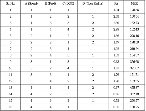
Table 2 Experimental table and its result

Sr. No. A (Speed) B (Feed) C (DOC) D (Nose Radius) Ra MRR

1 1 1 1 1 1.94 178.36

2 1 2 2 1 2.03 180.54

3 1 3 3 2 2.39 162.73

4 1 4 4 2 2.99 132.43

5 2 1 2 2 1.36 270.46

6 2 2 1 2 1.47 178.59

7 2 3 4 1 1.02 219.24

8 2 4 3 1 1.33 154.37

9 3 1 3 1 0.63 356.68

10 3 2 4 1 1.01 321.87

11 3 3 1 2 1.76 171.71

12 3 4 2 2 1.78 163.55

13 4 1 4 2 0.67 455.87

14 4 2 3 2 0.65 352.18

15 4 3 2 1 0.53 250.57

Data Analysis:

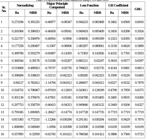
Table 3 Experimental result analyzed using PCA and GRA

Sr. No.

Normalizing Major Principle

Component Loss Function GR Coefficient

GRG

Ra MRR Ra MRR Ra MRR Ra MRR

1 0.273196 0.391255 -0.46977 -0.08347 0.944233 0.083468 0.3462 0.8569 0.6016

2 0.261084 0.396033 -0.46458 -0.09541 0.949418 0.095409 0.3450 0.8398 0.5924

3 0.221757 0.356976 -0.40916 -0.0956 1.004836 0.095599 0.3323 0.8395 0.5859

4 0.177258 0.290497 -0.3307 -0.08006 1.083297 0.080061 0.3158 0.8620 0.5889

5 0.389706 0.593279 -0.69497 -0.14393 0.71903 0.143926 0.4102 0.7765 0.5933

6 0.360544 0.39176 -0.53188 -0.02207 0.882121 0.02207 0.3618 0.9577 0.6597

7 0.519608 0.480923 -0.70737 0.02735 0.706625 0.02735 0.4144 0.9481 0.6813

8 0.398496 0.338633 -0.52115 0.042323 0.89285 0.042323 0.3590 0.9220 0.6405

9 0.84127 0.782412 -1.14794 0.041612 0.266057 0.041612 0.6527 0.9232 0.7879

10 0.524752 0.706067 -0.87019 -0.12819 0.543811 0.128189 0.4790 0.7959 0.6375

11 0.301136 0.376674 -0.47921 -0.05341 0.934788 0.053405 0.3485 0.9035 0.6260

12 0.297753 0.358759 -0.46415 -0.04313 0.949846 0.043132 0.3449 0.9206 0.6327

13 0.791045 1.000005 -1.26627 -0.14774 0.147728 0.147735 0.7719 0.7719 0.7719

14 0.815385 0.772535 -1.12266 0.030294 0.291341 0.030294 0.6318 0.9429 0.7874

15 1.000000 0.549649 -1.0956 0.318398 0.318398 0.318398 0.6109 0.6109 0.6109

16 0.557895 0.32959 -0.62745 0.161412 0.786548 0.161412 0.3886 0.7560 0.5723

Experimental data have been normalized. For surface roughness lower the better and for material removal rate higher the better criteria have been chosen. The normalized values are shown in the Table 3.

The Eigen analysis of the correlation Matrix is shown below. Eigenvalue 1.9801 0.0199

Ra 0.707 -0.707

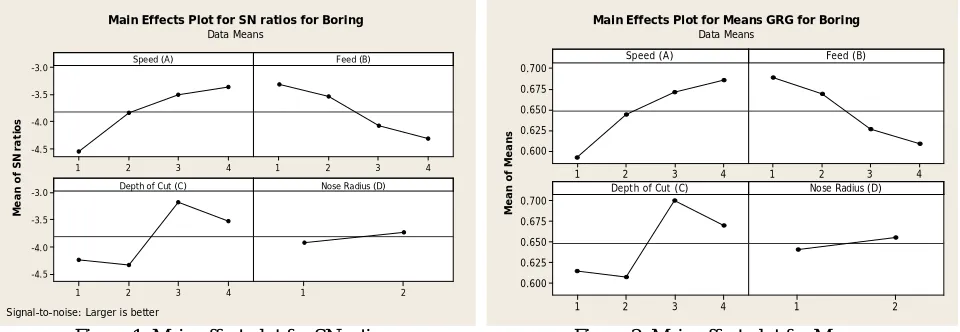
In order to eliminate response correlations, Principal component analysis has been applied to derive two independent quality indices called principal components. The independent quality indices are denoted as PC1 and PC2. Above represents the values of these independent principal components for 16 experimental runs. The major principal components, its loss function, grey relation co-efficient and grey relation grade are shown in table 3. Now the grey relation grade is main objective function and further analyzed data and the obtained results are shown in figure 1 &2.

4 3 2 1 -3.0 -3.5 -4.0 -4.5 4 3 2 1 4 3 2 1 -3.0 -3.5 -4.0 -4.5 2 1 Speed (A) M e a n o f S N r a ti o s Feed (B)

Depth of Cut (C) Nose Radius (D)

Main Effects Plot for SN ratios for Boring

Data Means

Signal-to-noise: Larger is better

Figure 1. Main effect plot for SN ration

4 3 2 1 0.700 0.675 0.650 0.625 0.600 4 3 2 1 4 3 2 1 0.700 0.675 0.650 0.625 0.600 2 1 Speed (A) M e a n o f M e a n s Feed (B)

Depth of Cut (C) Nose Radius (D)

Main Effects Plot for Means GRG for Boring

Data Means

Figure 2. Main effect plot for Means

From the above figure1 & 2, the optimal setting for multi objectives (For material removal rate and surface roughness) is A4B1C3D2. The response table for that is shown in table 4. From the response table and ANOVA we can say that depth of cut and speed are most significant parameters and nose radius is less significant parameters for selected multi quality characteristics. After applying the optimal setting of process parameters, confirmation test was carried out to validate the analysis. The improvement of the surface roughness ratio from the initial condition to the multi optimal condition is about 11% and reduced material removal rate approximately 7% from individual optimal condition. This PCA technique can be effectively applied for the optimization of multi-responses.

Table 4 Response Table for means of GRG

Levels Speed (A) Feed (B) Depth of Cut (C) Nose Radius (D)

1 0.5922 0.6887 0.6149 0.6405

2 0.5922 0.6692 0.6073 0.6557

3 0.6710 0.6260 0.7004

4 0.6856 0.6086 0.6699

Delta 0.0935 0.0801 0.0931 0.0152

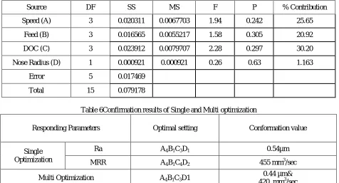
Table 5 ANOVA for multi objective characteristics (GRG)

Source DF SS MS F P % Contribution

Speed (A) 3 0.020311 0.0067703 1.94 0.242 25.65

Feed (B) 3 0.016565 0.0055217 1.58 0.305 20.92

DOC (C) 3 0.023912 0.0079707 2.28 0.297 30.20

Nose Radius (D) 1 0.000921 0.000921 0.26 0.63 1.163

Error 5 0.017469

Total 15 0.079178

Table 6Confirmation results of Single and Multi optimization

Responding Parameters Optimal setting Conformation value

Single Optimization

Ra A4B1C3D1 0.54µm

MRR A4B1C4D2 455 mm3/sec

Multi Optimization A4B1C3D1

0.44 µm& 420 mm3/sec

III.CONCLUSION

 The optimal quality parameters are mainly affected by depth of cut, spindle speed and feed rate. Nose radius has least effect on multi response parameters.

 From ANOVA analysis, parameters making significant effect on surface roughness are depth of cut, speed and feed with contribution of 30.20%, 25.65% and 20.92% respectively.

 The optimal process parameters in CNC TC are: speed of 1400 rpm, feed of 0.06 mm/rev, depth of cut of 1.4 mm and nose radius of 1.2 mm.

 The improvement of the surface roughness ratio from the initial condition to the multi optimal condition is about 11% and reduced material removal rate is approximately 7% from individual optimal condition.

REFERENCES

[1] MihirThakorbhai Patel, “Multi Objective Optimization Of Machining Parameters During Turning of E 250 B0 of Standard IS: 2062 Materialusing Grey Relation Analysis”, International Journal of Advanced Research in Engineering and Applied Sciences, Volume 4, No. 6, June 2015, pp. 57-71.

[2] Mihir T. Patel and Vivek A. Deshpande, “Optimization of Machining Parameters for Turning Different Alloy Steel Using CNC – Review”, International Journal of Innovative Research in Science, Engineering and Technology, Vol. 3, Issue 2, February 2014, pp. 9423 – 9430 (2). [3] Mihir Patel, “Optimization of Milling Process Parameters - A Review”, International Journal of Advanced Research in Engineering and

Applied Sciences, Volume 4, No. 9, September 2015, pp. 24 -37.

[4] Mihir Patel &HimanshuMevada, “Optimization of Turning Process Parameters by Different Optimization Technique- A Review”, International Journal of Advance Engineering and Research Development, Volume 2,Issue 3, March -2015, pp. 39-47.

[5] Johnson R.A., WichernD.W.,"Applied Multivariate Statistical Analysis", Prentice-Hall, Inc., Englewood Cliffs, New Jersey 07632, 2002. [6] RavinderKataria and Jatinder Kumar, “A comparison of the different multiple response optimization techniques for turning operation of AISI

O1 tool steel”, Journal of Engg. Research Vol. 2 No. (4), Dec 2014 pp. 161-184.

[8] Anish Nair and Dr. P Govindan, “Multiple Surface Roughness Characteristics Optimization in CNC End Milling of Aluminum using PCA”, International Journal Of Research In Mechanical Engineering & Technology, Vol. 3, Issue 2, May - Oct 2013, pp. 17-21.

[9] Milan Kumar Das, Kaushik Kumar, Tapan Kr. Barman and PrasantaSahoo, “Optimization of WEDM process parameters on EN31steel by weighted principal component analysis”, International Conference on Advances in Engineering & Technology – 2014 (ICAET-2014), pp. 30-33.

[10] RinaChakravorty, Susanta Kumar Gauri and Shankar Chakraborty, “A modified principal component analysis-based utility theory approach for optimization of correlated responses of EDM process”, International Journal of Engineering, Science and Technology, Vol. 4, No. 2, pp. 34-45, 2012.

[11] SanjitMoshat, SauravDatta, AsishBandyopadhyay and Pradip Kumar Pal, “International Journal of Engineering, Science and Technology, Vol. 2, No. 1, pp. 92-102, 2010.