Microarray Analysis of Replicate Populations Selected Against a
Wing-Shape Correlation in
Drosophila melanogaster
Kenneth E. Weber,*
,1Ralph J. Greenspan,
†David R. Chicoine,* Katia Fiorentino,*
Mary H. Thomas* and Theresa L. Knight*
*Department of Biological Sciences, University of Southern Maine, Portland, Maine 04104-9300 and†The Neurosciences Institute, San Diego, California 92121
Manuscript received October 18, 2007 Accepted for publication November 26, 2007
ABSTRACT
We selected bidirectionally to change the phenotypic correlation between two wing dimensions in Drosophila melanogasterand measured gene expression differences in late third instar wing disks, using microarrays. We tested an array of 12 selected lines, including 10 from a Massachusetts population (5 divergently selected pairs) and 2 from a California population (1 divergently selected pair). In the Massachusetts replicates, 29 loci showed consistent, significant expression differences in all 5 line-pair comparisons. However, the significant loci in the California lines were almost completely different from these. The disparity between responding genes in different gene pools confirms recent evidence that surprisingly large numbers of loci can affect wing shape. Our results also show that with well-replicated selection lines, of large effective size, the numbers of candidate genes in microarray-based searches can be reduced to realistic levels.
T
HE Drosophila wing is a convenient model system for shape genetics. Our approach has been to select against phenotypic correlations within the wing, using the metric of ‘‘angular offsets’’ (Weber 1990). Angular offsets reduce shape to its simplest quantifiable aspect—the allometric relation between two interland-mark distances—by measuring each individual’s deviation from the mean line of allometry of the base population (seematerials and methods). This converts variation that is orthogonal to the correlation into a univariate scale that is independent of size. Thus, angular offsets focus directly on the evolutionary constraints posed by correlations (Lande 1979) and quantify the breakage of these constraints (cf.Beldadeet al.2002).Many genes affect wing shape. Quantitative trait locus (QTL) mapping found at least 20 genes affecting one wing-shape trait in divergently selected lines from a wild sample (Weberet al.1999, 2001). Experimental selec-tion can change wing shape in many direcselec-tions (Weber 1990; Mezey and Houle 2005) and can affect small isolated parts (Weber1992). A screen of 50 randomP -element insertions found 11 insertions with rigorously validated wing-shape effects (Weber et al. 2005). In these cases, gene effects were in the range of 0.1–1 phenotypic standard deviations of the base population. These results show that the wing has a high short- and long-term potential to evolve new shapes based on many
existing alleles with small effects and many more loci that could mutate to produce such alleles. This suggests that replicate lines under identical selection might use different genes to produce similar changes in wing shape. Identical selection regimes often produce different genetic outcomes. In a classic example, Goodale(1941, 1953) selected for heavier mice and created a large-boned line, while Macarthur(1949) selected mice in the same way from a different stock and obtained a line that was not large boned, but obese. In another case (Swallowet al.1998; Houle-Leroyet al.2003), mice from a single stock were selected for wheel running in four replicate lines. All lines responded with compara-ble performance increases, but two distinct suites of physiological and morphological traits emerged. Cohan and Hoffmann(1986) selected for ethanol tolerance in Drosophila melanogaster from five locations along the North American West Coast and found that response occurred in genetically different ways. In these and other cases (e.g., Gromko 1995; Bult and Lynch 1996), replicate selection lines from different strains, or even from the same strain, produced the same selected phenotype by different genetic means.
On the other hand, identical selection often produces parallel genetic outcomes, even when starting with different strains or species. For example, in cereals like sorghum, rice, and maize, orthologous loci have been involved in parallel changes during domestication for traits such as large seeds and seasonal independence of flowering (Patersonet al.1995; Devos2005). Experi-ments with bacteriophages adapting to high
tempera-1Corresponding author:Department of Biological Sciences, University of
Southern Maine, 96 Falmouth St., Portland, ME 04104-9300. E-mail: [email protected]
ture (Bull et al. 1997; Wichman et al.1999) or toxic chemicals (Cunninghamet al.1997) show that identical selection in different lines can lead to parallel and sometimes almost identical changes in the same genes. Woodet al.(2005) review other cases of parallel genetic change in strains and species subjected to the same selective regime.
In adaptive radiations, parallel evolution often in-volves the same few major loci. Parallel morphological and genetic differences were found in independent cases of marine sticklebacks adapted to fresh water (Schluteret al.2004; Shapiroet al.2004), in species of Drosophila that independently evolved similar pigmen-tation of wings (Prud’hommeet al.2006) or abdomens (Gompel and Carroll 2003), and in beak length in Darwin’s finches (Abzhanov et al. 2006). Schluter et al.(2004) provide other examples both supporting and contradicting this principle.
In the most striking cases of genetic convergence, identical amino acid substitutions have occurred in the same proteins in unrelated groups (Patthy 1999; Carroll 2006). Yet when selection responses can be more fully dissected, genetic differences emerge. In cereal domestication, genetic parallelism is high in some traits but low in others (Galeand Devos1998; Morrell and Clegg 2007). In the bacteriophage studies (Wichmanet al.1999), loci with parallel changes were not those with the largest effects. In Drosophila, the same gene caused wing spots in independent lineages, but the regulatory modules were different (Prud’hommeet al.2006).
Genetic divergence or convergence during selection depends partly on population size and selection inten-sity and the nature of the selected trait. In the wheel-running study cited above, the alternative outcomes were attributed to drift in small populations, because they depended on the presence of a single allele with low frequency in the base population (Houle-Leroy et al.2003). Selection intensity may influence the rel-ative recruitment of major or minor genes (Lande 1983), as studies of the evolution of insecticide and herbicide resistance have emphasized (McKenzieet al. 1992; Gardner et al. 1998; Neve and Powles 2005). The primary determinant of genetic divergence or convergence may be the complexity of the trait. Fea-tures that utilize much information in development, and can be molded easily in many ways by selection, should permit alternative paths to similar phenotypes, and their responses in parallel selection lines should vary more. Wing shape seems to be such a trait.
In this study, we used microarrays to measure gene expression in the whole genome in a large panel of selection lines. The lines were created in different experiments, originated from separate populations, and included multiple replicates of one population, but all were created using the same selection regime and shape trait. Here we evaluate the data with two aims: (1)
to identify candidate wing-shape genes and (2) to assess variation in the outcome of identical selection regi-mes—between replicate lines from a single source and between lines from two geographically remote, local gene pools in Massachusetts and California.
MATERIALS AND METHODS
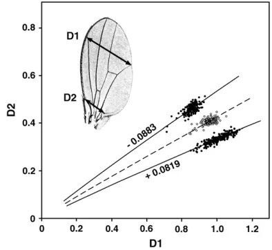
The trait and the selected lines:D1 and D2 are widths at the middle and base of the wing (Figure 1). The angular offset of a wing is the polar angle, in radians, between the point (D1, D2) and the point with equal radius (r) on the line of the polar equation u ¼ 0.4048r0.043 (males) or u ¼ 0.4148r0.134 (females). The polar equation is a curve approximating the mean allometric relation between D1 and D2, derived by regression of loguon logrin wild-type flies (Weber1990).
Clockwise and counterclockwise deviations from this baseline are called positive and negative, respectively. Angular offsets are independent of body size.
Lines H and L (Weber 1990) were created by divergent
selection of the most extreme 20% of 100 flies of each sex from a sample of a laboratory population established in 1981 from 350 isofemale lines captured in Lincoln, Massachusetts. The lines were selected for 20 generations, and all three major chromosomes were isogenized using balancer chromosomes. Lines H and L were then used to map QTL on chromosomes three (Weberet al.1999) and two (Weberet al.2001), usingin
situ-labeled insertion sites of the transposonrooas markers. Figure 2 outlines the creation of eight more selection lines. In September 1999, lines H and L were crossed in four separate crosses of 500 males and 500 virgin females to create Figure1.—Definition of the trait. The dashed line shows
the mean allometric relationship of D1 and D2 in wild-type males. The phenotype of each wing is the angular offset of its point (D1, D2) from this baseline in radians of rotation about the origin. Selection on this angle produces antagonis-tic changes in D1 and D2. The figure shows samples of male wings from a wild-type population (open circles), with a mean angular offset of approximately zero, and from two diver-gently selected populations (solid circles) with mean offsets of0.0883 and10.0819 radians (K. E. Weber, unpublished
the hybrid lines A, B, C, and D. Before crossing we verified that both H and L were still isogenic for all the sameroomarkers that were used in QTL mapping on all three main chromo-somes. Thus we can be certain that all hybrid populations began with identical fixed backgrounds and segregating alleles. Founder males and females were H and L, respectively, in A and B; C and D were the reciprocal cross.½About 10% of the phenotypic difference between H and L arises from the X chromosome (Weberet al.1999, 2001).For 34 generations,
each hybrid line was maintained in 30 vials with three female and five male parents per vial. In every generation, virgin offspring were collected for 9 days to include all eclosing flies, kept at 12°to prevent mating, and then randomly mated. Our aim was to mingle the H and L genomes in large panmictic populations with minimal selection.
After 34 generations of genetic mingling in these four hybrid lines, selection was reinitiated to derive a new pair of divergently selected lines from each hybrid line. The eight lines were designated A1, A2, B1, B2, and so on and were selected in the positive (1) or negative (2) direction. The parents were the most extreme 20% of 315 measured flies of each sex. In several generations fewer flies were measured, but the number of parents was always at least 63 of each sex per line. After 25 generations of selection, sublines were sib-mated for 10 generations to create inbred lines.
The California selected lines came from a base population that was derived from 40 D. melanogaster isofemale lines, captured in Davis, California, and kindly supplied by Michael Turelli (University of California, Davis, CA). In each genera-tion, the most extreme 20% of 200 individuals of each sex were selected as parents. After 21 generations of selection, the lines were inbred by sib-mating for 10 generations, then maintained in vial cultures for several years, and then further inbred by sib-mating for 10 more generations, prior to these experiments.
Staging and dissection of larvae: Culture vials were set up with potato-flake medium plus 0.05% bromphenol blue to obtain semisynchronous larvae. The blue medium was re-tained by late third instar larvae but gradually excreted, permitting visual staging (Maroniand Stamey1983; Andres
and Thummel1994). We selected larvae with a median time to
pupariation of 6.2 hr (data not shown). Larvae were dissected in cold PBS on siliconized slides using needle-tip tweezers, and wing disks were cleaned with tungsten needles. Each pair of disks was transferred to a tiny droplet of fresh PBS retained on the tip of a needle after dipping it in boiling deionized water
and then in ice-cold sterile PBS. Disks were transferred from this needle tip to the bottom of a 0.5-ml microcentrifuge tube in a covered gel-filled cooler (embedded in dry ice), where the droplet with disks was instantly frozen to the bottom. No damaged disks were used. Male and female larvae were not separated, so samples included both sexes about equally.
RNA was extracted (Dierick and Greenspan 2006) by
homogenization of 100 disks per sample, representing at least 50 larvae. Large samples of disks were used because individuals may vary greatly in expression levels (Oleksiaket al.2002). For
each sample, 90 culture vials were set up with blue medium and one mated female apiece. Only a few larvae came from each vial so any differences between cultures were averaged over many vials. Samples were analyzed using Affymetrix tech-nology (Drosophila Genome Array Version 2) according to the manufacturer’s protocols.
Statistical analysis of microarray data:The data set includes the scans of 36 Affymetrix Drosophila 2.0 microarray chips, representing six pairs of divergently selected lines and three samples per line. Results were analyzed using the software programs dChip (http://www.dchip.org; version of June 27, 2005), CyberT (Institute for Genomics and Bioinformatics, University of California, Irvine, CA), SAS and JMP5 (SAS Institute, Cary, NC), and Excel (Microsoft). Normalization of intensities and classification of probe sets as present, marginal, or absent by dChip was carried out anew within each subset of the data used in different tests. When line pairs were tested separately, the data for the six chips of each line pair were independently normalized using dChip and tested using a Bayesian analysis in CyberT after converting normalized inten-sities to natural logs. We used Bayesian methods fort-tests of individual line pairs because the sample sizes were small, with three chips for each selected line. For Bayesian statistical comparisons, variances were conditioned on the closest 50 probe sets above and below each probe set in order of their rank according to normalized intensity. Probabilities were corrected for the number of tests within each line pair by setting the significance threshold at 0.05/N, whereNwas the number of tested probe sets for that pair. Probe sets were also tested using the combined data for all five Massachusetts line pairs in nested ANOVAs, with chips nested within lines and lines within treatments, using natural log-transformed in-tensities in SAS to provide overall P-values for each probe set, similarly corrected for the total number of tests.
The raw array data files are available at http://www.ncbi. nlm.nih.gov/projects/geo/ under accession no. GSE9107.
Plan of data analysis: Our analysis began with two pre-liminary steps. First, we examined the entire data set to assess the consistency and quality of the normalized intensity data and the performance of the analysis software. We then screened the data for genes with zero expression (null alleles) either in one direction of selection or in one gene pool. These preliminary analyses indicated that the data were of consistent quality and that the main analysis could be based solely on comparisons of expression levels among transcribed genes (seeresultsfor details).
In the main analysis, our first aim was to identify a small number of high-quality candidate genes. We assumed that the Massachusetts lines had the same contributory genes since they all came from the same original sample, but the con-tributory genes in Massachusetts and California lines might be different. Therefore, we derived our candidate gene list solely from the Massachusetts lines, since we had five pairs of them but only one pair of California lines.
We had two criteria for candidate genes: our list includes only genes that were (1) consistently significant in all five Massachusetts line pairs, when each line pair was tested independently, and that were also (2) significant in the nested Figure2.—Derivation of lines. A wild Massachusetts
ANOVA of the combined Massachusetts data set. In the end, the candidate genes were completely decided by the first criterion, which was more stringent. This plan of analysis allowed us to use the same results to evaluate the incremental value of additional replicates, to investigate sources of varia-tion in the outcome of selecvaria-tion among lines, and to compare outcomes between the Massachusetts and California lines.
Estimation of centimorgan values: We created a look-up table to estimate locations of genes on the genetic map by entering the experimental centimorgan values listed by Ashburner in Lindsley and Zimm (1992, pp. 1117–1133)
and interpolating values for intervening genes. The centimor-gan values were plotted as a function of the starting nucleotide address for genes as given in the Affymetrix gene annotation list. Curves were fit to the data using the spline function in JMP5. The spline parameters of the best-fit curve for each major chromosome arm were:
X l¼5:00E116r2¼0:9995
2L l¼3:00E116r2¼0:9982
2R l¼3:00E117r2¼0:9986
3L l¼4:00E116r2¼0:9987
3R l¼2:00E116r2¼0:9997:
Calculations of heritabilities and effective factors: Herit-abilities and effective gene numbers were calculated for the four hybrid Massachusetts populations (A, B, C, and D) using the selection data (Falconerand Mackay1996). We
calcu-lated realized heritabilities for each of the eight derived selection lines by the method of Hill(1972) on the basis of
the first six generations of selection. We used the mean heritability of each pair of high and low lines to estimate the heritability of each hybrid population and the means of the two phenotypic standard deviations in the first generation of selection to estimate the standard deviation for each hybrid population. Total response was the difference between high and low lines after 25 generations of selection and 10 generations of inbreeding.
RESULTS
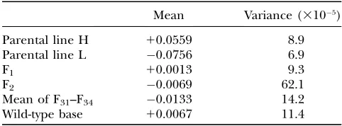
The phenotypic variances of isogenic lines H and L and of their four F1hybrids were all nearly equal (Table
1). In the F2generation, hybrid variance increased by a
factor of6, as large blocks of high and low selected alleles began to segregate. During 34 subsequent gen-erations of random mating in populations of an effec-tive size of180, mean hybrid variance declined almost to the same value as base population variance, indicat-ing approximate linkage equilibrium for alleles affect-ing the trait.
In generation F35, we began selecting divergently on
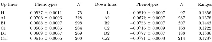
paired sublines from each hybrid line. After 25 gener-ations of selection, these new lines diverged about as much as the parental H and L lines and more in some cases (Table 2). Thus no significant genetic variation for the trait was lost during the 34 generations of hybrid mingling. After selection, the 8 new lines were sib-mated
for 10 generations to reduce genetic variation within lines. The two California lines were selected for 21 generations and then also inbred by sib-mating. Most of the phenotypic divergence between high and low lines remained after inbreeding. Tables 2 and 3 summarize the phenotypes of all 12 selected lines before and after inbreeding or, in the case of the H and L lines, before and after isogenization with balancers. The measure-ments in Table 3 were made just before microarray assays were performed on all lines.
Preliminary analysis of microarray data quality: On
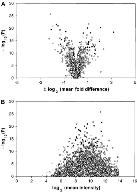
the Affymetrix chip, each probe is present in two ver-sions on contiguous spots: a 25-base version (PM) that is a perfect genomic match and another 25-base version (MM) with a single mismatch at the 13th base. A probe set includes 14 different paired PM/MM probes from one transcript, and the chip includes probe sets repre-senting mostD. melanogastertranscripts. The dChip soft-ware normalizes hybridization intensities across chips and classifies probe sets as present, absent, or marginal. A few probe sets that were called present had negative or zero intensities when evaluated as the sum of PM–MM differences. We eliminated these as well as Affymetrix control sequences. We then looked at several funda-mental aspects of the data after normalization by dChip across all 36 chips.
Figure 3A shows distributions of hybridization R -values, where R ¼ (PM MM)/(PM 1 MM) for all PM/MM probe pairs on all 36 chips (9.53106probe pairs) after separation into present, absent, and mar-ginal probe sets. In absent probe sets, Ris distributed symmetrically around zero, as expected for completely random hybridization. In the present probe sets,Rhas a primary mode on the positive side and a secondary mode showing a minor population of randomly hybrid-izing probe pairs within present probe sets. Figure 3B shows the distributions of probe sets on all 36 chips
TABLE 1
Means and variances of parental and hybrid Massachusetts lines
Mean Variance (3105)
Parental line H 10.0559 8.9
Parental line L 0.0756 6.9
F1 10.0013 9.3
F2 0.0069 62.1
Mean of F31–F34 0.0133 14.2
Wild-type base 10.0067 11.4
Means in radians of angular offset as defined inmaterials and methods. For lines H and L,N¼100. For generations
(6.8 3 105probe sets), according to the number of probe pairs (0–14) in each probe set showing the anomalous condition MM . PM for present, absent, and marginal probe sets. Again, present and absent calls are well differentiated, and the distribution for absent probe sets is that expected for random hybridization. Figure 3 shows that present and absent calls by dChip efficiently separated our probe sets into two distinct groups with appropriate distributions. Probe sets classi-fied as marginal were much more similar to absent probe sets than to present ones. We therefore did not include the marginal probe sets in our analysis.
We also asked how consistently each transcript was called present across all 36 chips. Figure 4 shows the distribution of all18,800 probe sets on the Affymetrix chip, according to the number of times each one was called present in 36 chips. Almost 7000 probe sets were called present on every chip. At the other extreme, 5000 probe sets were not called present even once. The remaining 36% of probe sets were present on some but not all chips. Thus the majority were either always present or never present.
The dChip notes recommend special attention to any chip where.5% of probe sets are classified as outliers. The average percentage of outliers per chip, among all 36 chips, was only 0.49% according to dChip. A single atypical chip (H-3) had 4.08% outliers.
Absent genes associated with lines or treatments:
Absent probe sets could be null expression alleles, which could be associated with trait variation. We first searched all 30 Massachusetts chips for probe sets that were called absent in one direction of selection but present in the other. We found only seven. Visual inspection of the PM/MM profiles in dChip showed that, in all cases, both the present and absent probe sets showed nearly identical profiles and essentially zero expression. These cases clearly represent random error in the evaluation of genes that are not actually expressed in the wing.
We next compared present and absent calls between Massachusetts and California to check for genes ex-pressed in one population and not the other. There are 10 possible comparisons between Massachusetts line pairs, with a mean of 7187 shared present probe sets (Table 4). There are five possible comparisons between the California line pair and the Massachusetts line pairs, with a mean of 7160 shared present probe sets. Since the within-population comparisons must represent a single group of probe sets and the between-population com-parisons show almost the same numbers, most present/ absent differences are probably due to random error.
We conclude that null expression alleles may not be important in the genetic variance of this trait. By eliminating absent genes from further comparisons TABLE 2
Mean phenotypes of all selected lines before inbreeding or isogenization
Up lines Phenotypes N Down lines Phenotypes N Ranges
H 0.053760.0011 75 L 0.081960.0007 97 0.1356
A1 0.070660.0006 328 A2 0.067260.0007 287 0.1378
B1 0.068860.0007 298 B2 0.075560.0007 307 0.1443
C1 0.050660.0006 284 C2 0.071660.0009 168 0.1222
D1 0.060960.0007 269 D2 0.077760.0007 183 0.1386
Ca1 0.051660.0006 200 Ca2 0.077160.0008 214 0.1287
Means and SE in radians of angular offset. Data are from selection generation 20 in H and L; 22 in Ca1 and Ca2, and 24 in line pairs A–D.Nis the sample size. All data are from males.
TABLE 3
Mean phenotypes of all selected lines after inbreeding or isogenization
Up lines Phenotypes N Down lines Phenotypes N Ranges
H 0.057560.0007 50 L 0.075160.0007 50 0.1326
A1 0.071160.0010 50 A2 0.066560.0013 50 0.1376
B1 0.066460.0009 50 B2 0.054560.0011 50 0.1209
C1 0.053460.0016 50 C2 0.063660.0014 50 0.1170
D1 0.068660.0010 50 D2 0.065060.0012 50 0.1336
Ca1 0.044960.0010 50 Ca2 0.065760.0012 50 0.1106
between populations or treatments, we simplified the rest of the analysis, which was focused on differences in expression intensity among genes called present on chips in both directions of selection or in both gene pools.
Transcripts associated with the trait in individual line
pairs:We began our main analysis by testing each line
pair separately. For each pair we tested probe sets for significant expression differences between high and low lines byt-test as explained inmaterials and methods. Table 5 shows the number of testable probe sets for each line pair and the number with significant expression differences, treating each line pair as an independent experiment and correcting for the number of tests in each pair. Testable probe sets included all for which at least two of the three samples were present in both the high and low line. This number was consistent with a range of 8346–8435. By contrast, the number of signif-icant probe sets was highly variable. We tested the numbers of nonsignificantvs. significant probe sets in Table 5 (R3C test of independence) to see whether the proportion of significant probe sets was independent of line pair. TheG-value was 268, with d.f. ¼ 5 and
P,1055. The lowP-value points to some factor or fac-tors with a large effect on the numbers of significant probe sets.
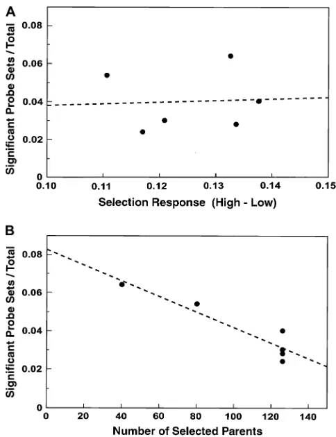
The effect of population size in selection: Figure 5
shows that the number of significant probe sets in line pairs is not correlated with phenotypic divergence, but may be influenced by the effective population sizes of lines during selection. Larger lines have fewer signifi-cant transcripts (r2¼0.872;P¼0.0067, assuming equal
variance at all population sizes). Perhaps alleles with no effect on the trait are more likely to be fixed in opposite directions by drift in smaller lines, but are controlled more by fitness selection in larger lines. The slope of the line in Figure 5B does not estimate the isolated effect of population size, because different base populations are included and because some reduction in the association of hitchhiking alleles with the trait would be expected in the derived lines even at the same population size. In any case, the four derived Massachusetts line pairs show a large, concerted decrease in significant probe sets compared to their parental lines, H and L. Yet they have approximately the same phenotypic divergence (Table 3). We conclude that many allelic differences that do not affect the trait were fixed oppositely in the parental lines and that in the larger, derived lines these differ-ences were more likely to be fixed for the same allele or to remain unfixed.
Consistency of significant probe sets in Massachusetts
lines: We next compared the five Massachusetts line
pairs to see how often the same probe sets were significant in different line pairs. Table 6 shows that 35 probe sets were significant in all five cases. Many more probe sets were significant in fewer than five. These were most numerous in the H/L lines, which were the par-ents of the other four pairs. For example, of 449 probe sets that were significant only once, almost half (218) were significant in the H/L comparison. Again, the greater abundance of significant transcripts in the H/L line pair is likely to be due to alleles that do not affect the trait. These alleles might have been separated from selected alleles by recombination in the hybrid Figure3.—Distributions of9.53106probe
pairs and6.8 3105probe sets from 36 chips. (A) Values of R for probe pairs in probe sets called present, absent, and marginal, whereR¼
populations with their larger size. This recombination could have occurred either during the 34 generations of mingling in the hybrid lines or during the 25 sub-sequent generations of selection.
Some probe sets that were significantly different in multiple line pairs showed expression differences that were in opposite directions in individual line pairs. That is, their expression was significantly higher in the high lineandsignificantly higher in the low line in different line pairs. The final column in Table 6 shows the num-ber of such cases. For example, of 164 probe sets that were significant in just two line pairs, 21 were significant in opposite directions. Overall,10% (39/375) of all probe sets that were significant more than once were expressed in opposite directions in different line pairs. For simplicity, we refer to these probe sets as ‘‘flip-flops.’’ They might be genes that are expressed oppositely in different epistatic complexes to produce equivalent phenotypic effects. A simpler explanation would be that they represent randomly fixed expression polymor-phisms with no relation to the trait.
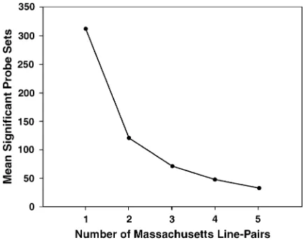
The value of additional replicates:We asked how the
number of consistently significant probe sets declines as
more replicates are added to the analysis. For this purpose we treated all five Massachusetts line pairs as replicates, representing approximately the same set of alleles and selection history. The average number of significant probe sets for individual Massachusetts line pairs in Table 5 is 312. Figure 6 shows that the addition of a second replicate line pair eliminated about two-Figure 4.—Distribution of probe sets according to the
number of chips on which each probe set was called present. Includes all Drosophila probe sets and Affymetrix control probe sets. Most probe sets were either always present or al-ways absent, indicating accurate detection.
TABLE 4
Consistently present probe sets within and between pairs of lines
Cal1/Ca2 H/L A1/A2 B1/B2 C1/C2 D1/D2
Ca1/Ca2 7527
H/L 7051 7346
A1/A2 7225 7111 7616 B1/B2 7151 7065 7258 7504 C1/C2 7190 7084 7290 7216 7524
D1/D2 7181 7099 7280 7233 7229 7547
Table includes probe sets called present in all 12 chips in each possible comparison of two line pairs.
TABLE 5
Testable and significant probe sets for each line pair
Line pair: H/L A1/A2 B1/B2 C1/C2 D1/D2 Ca1/Ca2
Testable probe sets
8350 8435 8367 8376 8405 8346
Significant probe sets
534 335 253 198 238 450
Probabilities were computed with log-transformed intensi-ties using Cyber-T with Bayesian methods and compared to P¼0.05/(testable probe sets in each line pair).
Figure5.—The proportion of significant probe sets within
thirds of significant probe sets, on average, by the criterion of consistent significance. The addition of a third replicate eliminated about half of the remaining probe sets. With the addition of more and more rep-licates, probe sets that remain consistently significant become increasingly interesting, but all probe sets would eventually be eliminated by the occurrence of occa-sional false negatives. According to Figure 6, in retro-spect, the critical or minimum number of replicate pairs of lines in our experiment was three. The addition of the fourth and fifth replicates was still possibly worth the effort in terms of the increasing resolution of probe sets. By extrapolation, a sixth replicate would be of marginal value.
Transposons:Transposons are disproportionately
fre-quent among the significant probe sets in Table 6, espe-cially among those with self-contradictory expression differences, described above as ‘‘flip-flops.’’ The total of 39 flip-flop probe sets in the final column of Table 6 includes at least 11 transposons. The two flip-flops that were significant in all five line pairs are both trans-posons. The large number of transposon flip-flops probably arises in part because transposons are present in numerous copies in the genome and most active insertion sites are not fixed. This allows their copy num-ber to diverge between selection lines. The divergence may be random or could be affected by hitchhiking due to associated genes for the trait. But not only flip-flops are transposons: among the 35 consistently significant probe sets in Table 6, 4 are transposons that show sig-nificant expression differences in the same direction of expression in all five line pairs. These four transposons, with their lengths and approximate copy numbers per genome according to FlyBase (Crosbyet al.2007), are hopper (1435 bp; 15), Rt1b (5100 bp; 40), 3S18
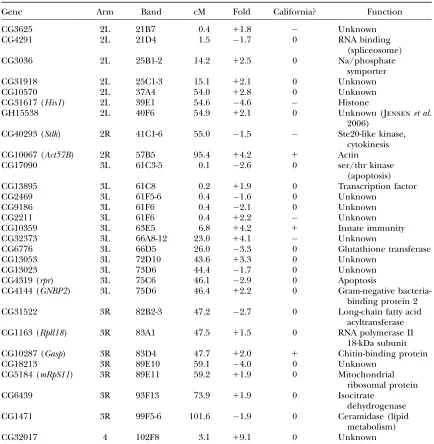
(6126 bp;20), andS(1736 bp;40). One interpreta-tion of such an associainterpreta-tion might be that the transposon itself affects the trait. It is also possible that these are cases where actively transcribed transposons are in-serted in genes that affect the trait in such a way that they create selectable alleles. This would mean that the insertion is a marker of a trait allele, but one that is dif-ficult to utilize in gene hunting because of the existence of many other copies of the same transposon. We re-moved all six transposons (two flip-flop, four non-flip-flop) from the list of 35 consistently significant probe sets, leaving 29 candidate genes for the trait. These are listed in Table 7 with some annotation according to FlyBase.
A test of the combined data:We regarded
indepen-dent significance in all five of five Massachusetts line pairs as a pragmatic first criterion for choosing candi-date genes. Genes that show such a consistent effect may be easier to validate. For a second, overall perspective, TABLE 6
Repeated significance of the same probe sets in Massachusetts replicates
Times significant Total H/L A1/A2 B1/B2 C1/C2 D1/D2 Opposite
5/5 35 35 35 35 35 35 2
4/5 78 74 66 57 54 61 6
3/5 98 89 60 46 35 64 10
2/5 164 118 78 45 31 56 21
1/5 449 218 96 70 43 22
Total 534 335 253 198 238
0/5 8541
Total probe sets tested: 9365
The first column gives the number of times a probe set was significant in the five comparisons. The final column gives the numbers of probe sets, included in the totals, that were significant multiple times but not always in the same direction (‘‘flip-flops’’).
Figure6.—As the number of replicate line pairs increases,
we combined the data from all five line pairs for all 7542 probe sets that were called present on at least two of three chips for every line and performed a nested ANOVA on the natural log-transformed intensities. Using a probability threshold corrected conservatively for the number of tests (P¼0.05/7542), there were 792 probe sets with significant expression differences, or just.10% of the genes commonly expressed in the wing
disk. Figure 7A shows a ‘‘volcano plot’’ of probabilityvs.
fold difference for the pooled Massachusetts data. The solid circles represent the 29 candidate genes from Table 7. Figure 7B shows the same probe sets and prob-abilities, plotted against log-transformed mean intensities. The candidate genes have reasonably strong intensi-ties and fold differences, with absolute fold differences of 1.5–9.1 and a mean of 2.8. In the ANOVA-based TABLE 7
Candidate genes from the Massachusetts lines
Gene Arm Band cM Fold California? Function
CG3625 2L 21B7 0.4 11.8 Unknown
CG4291 2L 21D4 1.5 1.7 0 RNA binding
(spliceosome)
CG3036 2L 25B1-2 14.2 12.5 0 Na/phosphate
symporter
CG31918 2L 25C1-3 15.1 12.1 0 Unknown
CG10570 2L 37A4 54.0 12.8 0 Unknown
CG31617 (His1) 2L 39E1 54.6 4.6 Histone
GH15538 2L 40F6 54.9 12.1 0 Unknown (Jensenet al.
2006)
CG40293 (Stlk) 2R 41C1-6 55.0 1.5 Ste20-like kinase,
cytokinesis
CG10067 (Act57B) 2R 57B5 95.4 14.2 1 Actin
CG17090 3L 61C3-5 0.1 2.6 0 ser/thr kinase
(apoptosis)
CG13895 3L 61C8 0.2 11.9 0 Transcription factor
CG2469 3L 61F5-6 0.4 1.6 0 Unknown
CG9186 3L 61F6 0.4 2.1 0 Unknown
CG2211 3L 61F6 0.4 12.2 Unknown
CG10359 3L 63E5 6.8 14.2 1 Innate immunity
CG32373 3L 66A8-12 23.0 14.1 Unknown
CG6776 3L 66D5 26.0 3.3 0 Glutathione transferase
CG13053 3L 72D10 43.6 13.3 0 Unknown
CG13023 3L 73D6 44.4 1.7 0 Unknown
CG4319 (rpr) 3L 75C6 46.1 2.9 0 Apoptosis
CG4144 (GNBP2) 3L 75D6 46.4 12.2 0 Gram-negative
bacteria-binding protein 2
CG31522 3R 82B2-3 47.2 2.7 0 Long-chain fatty acid
acyltransferase
CG1163 (Rpll18) 3R 83A1 47.5 11.5 0 RNA polymerase II
18-kDa subunit
CG10287 (Gasp) 3R 83D4 47.7 12.0 1 Chitin-binding protein
CG18213 3R 89E10 59.1 4.0 0 Unknown
CG5184 (mRpS11) 3R 89E11 59.2 11.9 0 Mitochondrial
ribosomal protein
CG6439 3R 93F13 73.9 11.9 0 Isocitrate
dehydrogenase
CG1471 3R 99F5-6 101.6 1.9 0 Ceramidase (lipid
metabolism)
CG32017 4 102F8 3.1 19.1 0 Unknown
Band locations and gene functions are according to FlyBase (Crosbyet al.2007). Centimorgans (cM) are
estimated as described inmaterials and methods. Fold differences from Massachusetts line means with sign
indicating greater expression in high lines (1) or low lines (). Entries under the column heading‘‘Califor-nia?’’ indicate whether the gene was not significant (0) in California lines, was significant in the same direction of expression (1), or was significant in the opposite direction (). FlyBase reports GH15538 only as a cDNA with an exact match on 2L coding for a putative protein. BLAST searches with the 14 Affymetrix probes for this detected transcript all give unique hits at this site. Jensenet al. (2006) report differential expression of GH15538
probability ranking of Figure 7, the 29 candidate genes are all highly significant, but some other probe sets look interesting as well. However, our immediate aim was to define a small preliminary set of the highest quality can-didates that would be the most likely to show detectable effects in a variety of tests. Our 29 candidate genes represent the intersection of two ranking methods. The first method emphasizes consistent association with the trait, while the second (Figure 7) allows for genes that may be less consistent but show significant overall asso-ciation with the trait. Each method may have pitfalls, but should be better than the other sometimes. Where both agree, the inference seems especially reliable.
Clustering among candidate genes:Table 7 indicates
the probable importance of hitchhiking. Five genes fall in an interval of 0.3 cM on the left end of chromosome three in division 61. Table 7 also includes two triplets and two pairs of closely linked genes (#0.5 cM). Clusters of linked, coexpressed genes have been found in Drosophila and other organisms (reviewed in Hurst et al.2004). However, every cluster in Table 7 includes genes that are expressed oppositely—some more in high lines and some more in low lines. Only two genes in one cluster are side by side (CG9186 and CG2211), but even these two are expressed oppositely with re-spect to the trait. The others are not adjacent, and most occur in regions of reduced recombination. For example, the 0.3-cM interval with five candidate genes covers 792 kbp containing 90 protein-coding genes. Despite their highly significant associations with the trait, some of the 29 candidate genes in tight clusters are likely to represent hitchhiking alleles that do not affect the trait.
We asked whether we would find larger clusters of genes associated with the trait if we relaxed our criteria to include more loci. We looked at the 200 most-significant probe sets in the list of 792 from the ANOVA of the Massachusetts lines, after eliminating all trans-posons. In addition to the 29 candidate genes, this larger group probably includes all expression differ-ences that contribute to the phenotypic divergence of the Massachusetts lines, and undoubtedly many that do not. Figure 8 shows how these 200 genes are distributed on the five main chromosome arms in bins of width 0.5 cM. For comparison, Figure 8 also shows the distribution of allD. melanogaster genes. In regions of low recombi-nation, the density of genes is lower on the physical map (Bartolome´ et al. 2002), but higher on the genetic map. The 200 candidate genes are not strongly clus-tered but are distributed over many sites, often as single, isolated genes. To some extent, their clustering reflects the overall distribution of gene densities.
Comparison of Massachusetts candidate genes to
significant California genes:We next compared the 29
final candidate genes from the Massachusetts data to the 450 probe sets that were significant in the single pair of divergent California lines (Table 5). The two groups had only eight genes in common, and five of these were flip-flops—significant in both the California and the Mas-sachusetts lines, but in opposite directions (column 6 in Table 7). Visual inspection of expression profiles in dChip confirmed that the California–Massachusetts flip-flop transcripts all show large expression differences that are associated consistently with the trait in all chips, but in opposite directions in the two populations. Again, various interpretations are possible for these flip-flop genes. They may affect the trait in a context-dependent way that is opposite in the two genetic backgrounds. They may also be cosmopolitan expression polymor-phisms that do not affect the trait in either population. Figure7.—Probabilityvs.fold difference and intensity in
Three of them occur in gene clusters in Table 7, strongly suggesting fixation by hitchhiking in the Massachusetts lines. Overall, the California data give virtually no sup-port to the candidate genes that we would choose by the criteria that we applied to the Massachusetts data. The simplest explanation is that the wing-shape genes seg-regating in these populations were very different.
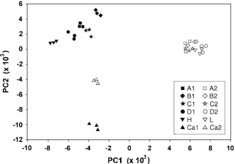
Visualizing the differences between gene pools:The
Massachusetts and California data sets showed large differences in loci associated with the trait. To study these differences further, we pooled and ranked both data sets separately by t-test probabilities, using the 7000 probe sets called present on every one of the 36 chips, and then compared the 1000 probe sets with the Figure 8.—Genetic map
lowestP-values for each population. Of these, only 208 were the same for both populations. (In random draws of 1000 from 7000, 143 would be the same.) We combined these probe sets from both populations for a total of 2000 208 ¼ 1792. The chips from both populations were renormalized as a group in dChip, so that we could perform a principal components analysis (PCA) using these 1792 probe sets, with the probe sets as objects and the 36 chips as variables, to visualize the associations between chips. The first two components of variation explained 49.8% of the variance. In Figure 9, each line is represented by three replicate chips that form a tight cluster. The 10 Massachusetts lines form distinct clusters of high lines and low lines, differenti-ated along the first principal component, and the high lines are more dispersed than the low lines. The two California lines are differentiated along the second principal component. California and Massachusetts genes clearly show different associations with the trait.
Differences between replicate lines within treatments:
The derived Massachusetts line pairs came from
repli-cate crosses of two isogenic lines (H and L), thus creat-ing hybrid lines with identical segregatcreat-ing alleles and identical fixed genetic backgrounds. We asked how much genetic differentiation occurred between them in each direction of selection. These lines are represented by 833¼24 chips and 7048 probe sets that were present on every chip. For each probe set, we tested the variance in expression among lines over the variance among chips within lines, within each direction of selection, by ANOVA. We found significant variances (i.e.,P # 0.05, without correcting for the total number of ANOVAs) among high-line means for 34.4% of all probe sets and among low-line means for 21.9% of all probe sets. This result agrees with the PCA analysis (Figure 9), showing chips highly clustered within differentiated lines and greater differentiation among high lines than low lines. The percentages seem huge compared to the expectation of 5% of all probe sets. However, they evidently reflect the random fixation of many segregating effects on gene expression that do not affect the trait. Alleles that do not affect a selected trait will often be fixed inconsistently among lines selected in the same direction.
Effective number of contributory loci:We calculated
realized heritabilities and effective gene numbers for the four hybrid Massachusetts lines from the selection data. The formula assumes that all allele frequencies were 0.5 when selection began—a reasonable approxi-mation since the lines were hybrids of two isogenic lines and were maintained at large size. The formula also assumes that alleles were fixed in the high and low selected lines, so we used the phenotypes of the selected lines after inbreeding. The estimates of gene number were fairly consistent. The closeness between the mean estimated gene number of Table 8 (26.5) and the number of candidate genes in Table 7 (29) owes much to chance. But the result may indicate that our previous estimate of 20 detectable genes for this trait, from QTL mapping of the Massachusetts H and L lines, was not too far off (Weberet al.1999, 2001).
DISCUSSION
We identified candidate genes for a wing-shape trait by microarray expression analysis of divergent selection Figure9.—Principal components analysis showing
cluster-ing of all 36 chips along the first two components of variance, according to the 1792 probe sets with lowest the P-values. Solid symbols, high lines; open symbols, low lines. For each line, three replicate samples (individual chips) are tightly clustered. The five Massachusetts low lines are clustered more closely than the five high lines. Massachusetts and California lines diverge orthogonally for the probe sets associated most closely with the trait by their expression differences.
TABLE 8
Calculation of effective gene numbers for the derived Massachusetts lines
Line pair h26SE Response (radians) Sp Rp¼response/Sp ne¼Rp2/8h2
A1/A2 0.5960.05 0.1376 0.012 11.47 27.9
B1/B2 0.3860.03 0.1209 0.013 9.30 28.5
C1/C2 0.4560.10 0.1170 0.013 9.00 22.5
D1D2 0.4960.05 0.1336 0.013 10.28 27.0
Realized heritability (h2) was calculated as explained inmaterials and methods. ‘‘Response’’ is the
lines. The lines were replicated within one population and also between two distant locations. The genetic outcomes of selection were variable both within and between gene pools. The results confirm the highly polygenic and degenerate basis of wing shape and shed light on the use of microarrays with selection lines to find quantitative trait genes.
Our data suggest that large population size usefully reduces the number of genes identified as candidates in selected lines by reducing the fixation of alleles with no effect on the trait. The parental lines (H and L) showed 534 significant loci (Table 5), but the hybrid lines derived from them had far fewer (198–335), despite having almost the same phenotypic divergence (Table 3). We attribute this difference to reduced fixation of noncontributory alleles due to recombination in the hybrid lines. This was probably enhanced by their larger size: lines H and L had 40 selected parents per line during selection, whereas the hybrid lines had 126. Selection is more deterministic in larger populations, and more efficient in sorting additive effects. This should reduce variation among outcomes and the number of significant genes.
Resolution was also improved by the replication of selection lines (Figure 6). When tested separately, the individual line pairs all showed unrealistically high numbers of significant probe sets (Table 5). But many probe sets were significant in only one line pair or in several (Table 6). Genes that were significant in some comparisons, but not in all, in some cases would be genes of lesser effect that were not consistently fixed, but many of them must simply be randomly fixed genes with no effect on the trait. Random fixation and hitchhiking are inevitable in finite selection lines. As many as four or five pairs of replicate selection lines may be useful in eliminating these false positives and genes with marginal or inconsistent effects.
A problem with our method of replication may be that the derived Massachusetts replicates represented too few recombinant haplotypes, because of the way in which they were constructed from crosses of isogenic lines. This is almost certainly the reason that we found some tightly linked clusters of genes showing the same repeated association with the trait. Even after 34 generations of hybrid mingling, and even after the trait variance declined to nearly base population levels, the originally isogenic H and L genomes would not dissolve into global linkage equilibrium. Many tight linkages persisted in the same phase in all lines. The same problem will occur whenever replicates come from a restricted source. Residual linkage disequilibrium will preserve numerous blocks of alleles in the same phase that have no effect on the trait, and this will inflate the number of significant genes, even in the combined analysis. Thus replicates for gene hunting should arise from wide sampling within a gene pool. Yet our results also suggest a potential dilemma: if sampling comes
from locations that are too far apart, results may be inconsistent because different contributory alleles are present.
Nevertheless, selection lines from distant gene pools may also play a role when looking for genes in highly polygenic traits. We found five genes that were signifi-cant in opposite directions in the Massachusetts and California lines. These may be ubiquitous expression polymorphisms, unrelated to the trait. Even after com-ing up ‘‘significant’’ five times in the Massachusetts lines, an allele might be associated with the trait only because it is closely linked to some other allele (not necessarily an expression polymorphism) and always in the same phase. The California results flag the flip-flop candidate genes as potential false positives, although worthy of investigation.
More interesting than these flip-flops is the finding that virtually no genes with significant expression differ-ences were associated with the trait in thesamedirection of expression in both Massachusetts and California flies. This result is credible because the replicated Massachu-setts lines do agree with each other, showing a substan-tial core group of consistently significant genes. This repeatability proves the reliability of the microarray mea-surements. Equally convincing is the close agreement between chips within lines, since each chip represents an independent sample of disks. By the same token, the striking disparity between the Massachusetts and Cal-ifornia lines—all tested simultaneously—must be a real phenomenon. This result argues that most expression differences with important effects on this trait are dif-ferent in the two gene pools. Several recent studies sup-port this interpretation.
In a screen of 50 random homozygous-viable P -element insertions, 11 (22%) had significant and re-peatable effects on wing shape (Weberet al.2005). All 11 were in sites that would be likely to cause expression differences in associated genes. The sample is small, but if it is even approximately representative, then the total number of genes in the genome that can affect wing shape by changes in expression is vastly greater than the number that could be segregating in any local popula-tion sample. This implies that, in populapopula-tion samples from widely separated locations, most genes that con-tribute to selection response for wing-shape traits might be different, as we report here.
QTL analyses of genetic variation for wing shape are also consistent with this conclusion. Wing-shape QTL have now been mapped in three different labs using different genetic stocks and trait definitions (Weber et al. 1999, 2001; Zimmerman et al. 2000; Mezey et al. 2005). A comparison of all three studies concluded that, although each one detected many wing-shape genes, the loci in each study were probably mostly different (Mezeyet al.2005).
Our QTL map for lines H and L (Weber et al. 1999, 2001) was a continuum of broad overlapping probability peaks, with QTL assigned at high points. Some points fall within 0.5 cM of the candidate genes in Table 7, but locations are only approximate, and, in regions of aver-age gene density, 0.5 cM can include 25 genes. More-over, genes that could affect wing shape are not obvious from their known features (Weberet al. 2005).
The candidate genes that we identified in the Massachusetts lines show a notable lack of coincidence with any of the 213 genes previously associated with non-neural aspects of wing development (Brody 2005), including genes implicated in regulating wing shape through cell proliferation such as vestigial (Kim et al. 1996; Baena-Lopezand Garcia-Bellido2006),Notch, orDelta(Baonzaand Garcia-Bellido2000). They in-clude none of the 43 genes in the transforming growth factor-band epidermal growth factor signaling pathways tested by Dworkinand Gibson(2006), the majority of which have small effects on wing shape. Of the 11 genes affecting wing shape in ourP-element screen (Weber et al. 2005), one (hephaestus) coincided with a known wing developmental mutant and one (stet) showed shape effects in the survey of Dworkinand Gibson(2006).
There could be many reasons for the differences be-tween our results and those of previous mutation studies. Perhaps genes previously identified as major mutants were involved in our experiments but their expression differences were too small to be significant. Or perhaps some classical developmental genes affect the timing or location of transcription without changing mean ex-pression levels in disks in the stage at which we assayed them. It is clear that some morphological traits are influenced by many genes with small effects (Norga et al.2003; Mezeyet al.2005; Weberet al.2005), and this fact alone may account for the lack of extensive overlap of wing-shape genes identified by different approaches. Several of the genes in Table 7 affect functions that could be relevant to wing development, including the well-studied cell death genereaper(Whiteet al.1996), theCG17090gene with homology to serine/threonine protein kinases associated with apoptosis, and the Ste20 kinase-like geneStlkassociated with cytokinesis in yeast (Cvrckovaet al. 1995). Three other genes are associ-ated with the regulation of gene expression: the RNA polymerase subunitRpll18, the histone geneHis1, and a putative RNA-binding protein component of the spli-ceosomeCG4291. Others with possible developmental relevance include the cytoskeletal actin geneAct57Band two genes associated with lipid biosynthesis (CG31522
andCG1471).
There is one striking correspondence between the present results and the 11 genes with shape effects caused byP-element insertions in Weberet al.(2005). None of those 11 genes were significant in this study, but 10 of them were among the 6843 transcripts that were called present on all 36 chips. This result is extremely
nonrandom. It makes sense because Weberet al.(2005) was a loss-of-function screen, where insertions affecting wing shape should occur in genes that are normally expressed in wing disks. Shape changes may also arise by ectopic expression of genes not normally active in wings. But from this coincidence of results, and other results reported here, it appears that selection has ample scope to act simply by modulating the expression of active genes. These genes are expressed at different intensities in localized regions of wing disks (Butler et al.2003), but most are expressed not only in wings but also in all imaginal disks (Klebeset al.2002).
In our view, selection penetrates an ever-expanding field of potential variation, with incremental improve-ments of trait alleles (Weberet al.2005) and progressive transfer of selection to modifier genes (Weber1996). This is enhanced by the degenerate and network nature of ways in which genes influence phenotypes (Greenspan 2001, 2004; Dworkinand Gibson2006). In some traits, alleles may affect a trait inconsistently in different ge-netic backgrounds (Van Swinderen and Greenspan 2005). In such cases, microarray analysis of replicated selection lines might be used to seek Wrightian peaks in the genetics of quantitative traits. However, the amount of replication and validation that may be required to achieve definitive results is still daunting. On the other hand, if any of our flip-flop genes prove to have opposite effects in different genetic backgrounds, we will have a case worth further study.
Microarray analysis of divergently selected lines is an established method of gene hunting (Tomaet al.2002; Mackay et al. 2005; Dierick and Greenspan 2006; Edwards et al.2006). The use of more replicate lines can greatly increase resolution by eliminating many false candidates caused by random fixation and hitchhiking. Replicates should have the same genetic base, but also the likelihood of high recombinational diversity among replicates. Larger populations may also help improve resolution. The consistency of recent results shows that microarray expression measurements are reliable. With further development of methods, microarray testing of replicated selection lines should become increasingly efficient in the search for quantitative trait genes.
Thanks go to L. Harshman and two anonymous reviewers for comments on the manuscript. This work was supported by the National Science Foundation under grant no. DEB-0344003 to K.E.W. and grant no. 0432063 to R.J.G. R.J.G. is the Dorothy and Lewis B. Cullman Fellow at the Neurosciences Institute, which is supported by the Neurosciences Research Foundation.
LITERATURE CITED
Abzhanov, A., W. P. Kuo, C. Hartmann, B. R. Grant, P. R. Grant
et al., 2006 The calmodulin pathway and evolution of elongated beak morphology in Darwin’s finches. Nature442:563–567. Andres, A. J., and C. S. Thummel, 1994 Methods for quantitative
(Methods in Cell Biology, Vol. 44), edited by L. G and E. Fyrberg. Academic Press, San Diego.
Baena-Lopez, L. A., and A. Garcia-Bellido, 2006 Control of
growth and positional information by the graded vestigial expres-sion pattern in the wing ofDrosophila melanogaster.Proc. Natl. Acad. Sci. USA103:13734–13739.
Baonza, A., and A. Garcia-Bellido, 2000 Notch signaling directly
controls cell proliferation in the Drosophila wing disc. Proc. Natl. Acad. Sci. USA97:2609–2614.
Bartolome´, C., X. Masideand B. Charlesworth, 2002 On the
abundance and distribution of transposable elements in the ge-nome of Drosophila melanogaster. Mol. Biol. Evol.19:926–937. Beldade, P., K. Koopsand P. M. Brakefield, 2002 Developmental
constraints versus flexibility in morphological evolution. Nature 416:844–847.
Brody, T., 2005 The Interactive Fly. http://rail.bio.indiana.edu/
allied-data/lk/interactive-fly/aimain/1aahome.htm.
Bull, J. J., M. R. Badgett, H. A. Wichman, J. P. Huelsenbeck, D. M.
Hilliset al., 1997 Exceptional convergent evolution in a virus.
Genetics147:1497–1507.
Bult, A., and C. B. Lynch, 1996 Multiple selection responses in
house mice bidirectionally selected for thermoregulatory nest-building behavior: crosses of replicate lines. Behav. Genet.26: 439–446.
Butler, M. J., T. L. Jacobsen, D. M. Cain, M. G. Jarman, M. Hubank
et al., 2003 Discovery of genes with highly restricted expression patterns in theDrosophilawing disc using DNA oligonucleotide microarrays. Development130:659–670.
Carroll, S. B., 2006 The Making of the Fittest.W. W. Norton, New York.
Cohan, F. M., and A. A. Hoffmann, 1986 Genetic divergence under
uniform selection. II. Different responses to selection for knock-down resistance to ethanol amongDrosophila melanogaster popu-lations and their replicate lines. Genetics114:145–163. Crosby, M. A., J. L. Goodman, V. B. Strelets, P. Zhang, W. M.
Gelbartet al., 2007 FlyBase: genomes by the dozen. Nucleic
Acids Res.35:D486–D491.
Cunningham, C. W., K. Jeng, J. Husti, M. Badgett, I. J. Molineux
et al., 1997 Parallel molecular evolution of deletions and non-sense mutations in bacteriophage T7. Mol. Biol. Evol.14:113–116. Cvrckova, F., C. De Vergilio, E. Manser, J. R. Pringle and K.
Nasmyth, 1995 Ste20-like protein kinases are required for
normal localization of cell growth and for cytokinesis in budding yeast. Genes Dev.9:1817–1830.
Devos, K. M., 2005 Updating the ‘‘crop circle.’’ Curr. Opin. Plant
Biol.8:155–162.
Dierick, H. A., and R. J. Greenspan, 2006 Molecular analysis of flies
selected for aggressive behavior. Nat. Genet.38:1023–1031. Dworkin, I., and G. Gibson, 2006 Epidermal growth factor
recep-tor and transforming growth facrecep-tor-bsignaling contributes to var-iation for wing shape inDrosophila melanogaster. Genetics 173: 1417–1431.
Edwards, A. C., S. M. Rollmann, T. J. Morganand T. F. C. Mackay,
2006 Quantitative genomics of aggressive behavior in Drosoph-ila melanogaster. PLoS Genet.2(9): e154.
Falconer, D. S., and T. F. C. Mackay, 1996 Introduction to
Quantita-tive Genetics.Longman, Harlow, UK.
Gale, M. D., and K. M. Devos, 1998 Plant comparative genetics
af-ter 10 years. Science282:656–659.
Gardner, S. N., J. Gresseland M. Mangel, 1998 A revolving dose
strategy to delay the evolution of both quantitative vs. major mon-ogene resistances to pesticides and drugs. Int. J. Pest Manage.44: 161–180.
Gompel, N., and S. B. Carroll, 2003 Genetic mechanisms and
con-straints governing the evolution of correlated traits in drosophil-id flies. Nature424:931–935.
Goodale, H. D., 1941 Progress report on possibilities in
progeny-test breeding. Science94:442–443.
Goodale, H. D., 1953 Appendix: third progress report on breeding
larger mice, in A study of selection limits in the mouse, D. S. Falconerand J. W. B. King. J. Genet.51:561–581.
Greenspan, R. J., 2001 The flexible genome. Nat. Rev. Genet.2:
383–387.
Greenspan, R. J., 2004 E pluribus unum, ex uno plura:
quantitative-and single-gene perspectives on the study of behavior. Annu. Rev. Neurosci.27:79–105.
G , M. H., 1995 Unpredictability of correlated responses to se-lection: pleiotropy and selection interact. Evolution49:685–693. Hill, W. G., 1972 Estimation of realized heritabilities from selection
experiments. II. Selection in one direction. Biometrics28:767– 780.
Houle-Leroy, P., H. Guderley, J. G. Swallowand T. Garland, Jr.,
2003 Artificial selection for high activity favors mighty mini-muscles in house mice. Am. J. Physiol. Regul. Integr. Comp. Phys-iol.284:433–443.
Hurst, L. D., C. Pa´ land M. J. Lercher, 2004 The evolutionary
dy-namics of eukaryotic gene order. Nat. Rev. Genet.5:299–310. Jensen, H. R., I. M. Scott, S. R. Sims, V. L. Trudeauand J. T. Arnason,
2006 The effect of a synergistic concentration of aPiper nigrum
extract used in conjunction with pyrethrum upon gene expression inDrosophila melanogaster.Insect Mol. Biol.15:329–339. Kim, J., A. Sebring, J. J. Esch, M. E. Kraus, K. Vorwerk et al.,
1996 Integration of positional signals and regulation of wing formation and identity byDrosophila vestigialgene. Nature382: 133–138.
Klebes, A., B. Biehs, F. Cifuentes, and T. B. Kornberg, 2002
Ex-pression profiling of Drosophila imaginal discs. Genome Biol. 3(8): RESEARCH0038.1–0038.16
Lande, R., 1979 Quantitative genetic analysis of multivariate
evolu-tion, applied to brain:body size allometry. Evolution33:402–416. Lande, R., 1983 The response to selection on major and minor
mu-tations affecting a metrical trait. Heredity50:47–65.
Lindsley, D. L., and G. G. Zimm, 1992 The Genome of Drosophila
mel-anogaster.Academic Press, San Diego.
Macarthur, J. W., 1949 Selection for small and large body size in
the house mouse. Genetics34:194–209.
Mackay, T. F. C., S. L. Heinsohn, R. F. Lyman, A. J. Moehring, T. J.
Morganet al., 2005 Genetics and genomics ofDrosophila
mat-ing behavior. Proc. Natl. Acad. Sci. USA102:6622–6629. Maroni, G., and S. C. Stamey, 1983 Use of blue food to select
syn-chronous, late third-instar larvae. Dros. Inf. Serv.59:142–143. McKenzie, J. A., A. G. Parkerand J. L. Yen, 1992 Polygenic and
sin-gle gene responses to selection for resistance to diazinon in Lu-cilia cuprina.Genetics130:613–620.
Mezey, J. G., and D. Houle, 2005 The dimensionality of genetic
var-iation for wing shape in Drosophila melanogaster. Evolution59: 1027–1038.
Mezey, J. G., D. Houleand S. V. Nuzhdin, 2005 Naturally
segregat-ing quantitative trait loci affectsegregat-ing wsegregat-ing shape ofDrosophila mela-nogaster.Genetics169:2101–2113.
Morrell, P. L., and M. T. Clegg, 2007 Genetic evidence for a
sec-ond domestication of barley (Hordeum vulgare) east of the Fertile Crescent. Proc. Natl. Acad. Sci. USA104:3289–3294.
Neve, P., and S. Powles, 2005 Recurrent selection with reduced
her-bicide rates results in the rapid evolution of herher-bicide resistance inLolium rigidum.Theor. Appl. Genet.110:1154–1166. Norga, K. K., M. C. Gurganus, C. L. Dilda, A. Yamamoto, R. F.
Lymanet al., 2003 Quantitative analysis of bristle number in
Drosophila mutants identifies genes involved in neural develop-ment. Curr. Biol.13:1388–1396.
Oleksiak, M. F., G. A. Churchilland D. L. Crawford, 2002
Vari-ation in gene expression within and among natural populVari-ations. Nat. Genet.32:261–266.
Paterson, A. H., Y.-R. Lin, Z. Li, K. F. Schertz, J. F. Doebleyet al.,
1995 Convergent domestication of cereal crops by independent mutations at corresponding genetic loci. Science269:1714–1718. Patthy, L., 1999 Protein Evolution. Blackwell Science, Oxford.
Prud’homme, B., N. Gompel, A. Rokas, V. A. Kassner, T. M.
Williamset al., 2006 Repeated morphological evolution through
cis-regulatory changes in a pleiotropic gene. Nature440:1050– 1053.
Schluter, D., E. A. Clifford, M. Nemethyand J. S. McKinnon,
2004 Parallel evolution and inheritance of quantitative traits. Am. Nat.163:809–822.
Shapiro, M. D., M. E. Marks, C. L. Peichel, B. K. Blackman, K. S.
Nerenget al., 2004 Genetic and developmental basis of
evolu-tionary pelvic reduction in threespine sticklebacks. Nature428: 717–723.
Swallow, J. G., P. A. Carterand T. Garland, Jr., 1998 Artificial
Toma, D. P., K. P. White, J. Hirsch and R. J. Greenspan,
2002 Identification of genes involved inDrosophila melanogaster
geotaxis, a complex behavioral trait. Nat. Genet.31:349–353. VanSwinderen, B., and R. J. Greenspan, 2005 Flexibility in a gene
network affecting a simple behavior inDrosophila melanogaster. Ge-netics169:2151–2163.
Weber, K. E., 1990 Selection on wing allometry inDrosophila
mela-nogaster.Genetics126:975–989.
Weber, K. E., 1992 How small are the smallest selectable domains of
form? Genetics130:345–353.
Weber, K. E., 1996 Large genetic change at small fitness cost in large
populations of Drosophila melanogaster selected for wind-tunnel flight: rethinking fitness surfaces. Genetics144:205–213. Weber, K., R. Eisman, L. Morey, A. Patty, J. Sparkset al., 1999 An
analysis of polygenes affecting wing shape on chromosome 3 in
Drosophila melanogaster.Genetics153:773–786.
Weber, K., R. Eisman, S. Higgins, L. Morey, A. Patty et al.,
2001 An analysis of polygenes affecting wing shape on
chro-mosome 2 in Drosophila melanogaster. Genetics 159: 1045– 1057.
Weber, K., N. Johnson, D. Champlinand A. Patty, 2005 ManyP
-element insertions affect wing shape inDrosophila melanogaster.
Genetics169:1461–1475.
White, K., E. Tahaogluand H. Steller, 1996 Cell killing by the
Drosophila genereaper.Science271:805–807.
Wichman, H. A., M. R. Badgett, L. A. Scott, C. M. Boulianneand J.
J. Bull, 1999 Different trajectories of parallel evolution during
viral adaptation. Science285:422–424.
Wood, T. E., J. M. Burkeand L. H. Rieseberg, 2005 Parallel
geno-typic adaptation: when evolution repeats itself. Genetica 123: 157–170.
Zimmerman, E., A. Palssonand G. Gibson, 2000 Quantitative trait
loci affecting components of wing shape inDrosophila melanogaster.
Genetics155:671–683.