Probabilistic and Nondeterministic Systems

SONI, ARVIND. Probabilistic and Nondeterministic Systems . (Under the direction of Professor Dr. S. Purushothaman Iyer).

Probabilistic and nondeterministic systems are important to model systems such as distributed network protocols, concurrent systems and randomized algorithms, where nondeterminism is inherently present along with probabilistic choices. Probabilistic transi-tion systems without any nondeterminism have been explored over the past decade. Several logics have been proposed to express the probabilistic behavior of systems. Nondetermin-istic systems differ from their probabilNondetermin-istic counterparts in that there behavior needs a notion of scheduler which resolves the nondeterministic choices. The probability space of observations of such systems is dependent on the choice of scheduler. In the absence of unique probability space the system properties can only be measured in intervals. The methods proposed in literature for quantitative analysis of nondeterministic systems use approximations for conjunction and disjunction to avoid the nonlinearity in the equations for measures.

by

Arvind Soni

A thesis submitted to the Graduate Faculty of North Carolina State University

in partial satisfaction of the requirements for the Degree of

Master of Science

Department of Computer Science

Raleigh 2004

Approved By:

Dr. George N. Rouskas Dr. Ting Yu

Biography

Acknowledgements

This thesis wouldn’t have been possible without the support and guidance of my adviser, Dr. Purushothaman Iyer, who with a great deal of patience and kindness helped me through out the duration of this work. Many thanks to Burak Serdar, for his timely help on various occasions.

Contents

List of Figures vii

List of Tables viii

1 Introduction 1

1.1 Contributions . . . 2

2 Probabilistic-Nondeterministic Systems 4 2.1 Models . . . 4

2.1.1 Measure space . . . 9

3 Extended Generalized Probabilistic Logic 10 3.1 Syntax of EGPL . . . 11

3.2 Semantics of EGPL . . . 11

4 Model Checking of PNS 15 4.1 Outline of the approach . . . 15

4.2 Graph Construction . . . 16

4.3 Generating constraints from the graph . . . 19

4.4 Model Checking Example . . . 20

5 Implementation and Case Studies 23 5.1 Quantitative Model Checker . . . 24

5.2 Randomized Self-Stabilizing Protocol(RSSP) . . . 24

5.2.1 Abstraction based model . . . 26

5.2.2 Experimental Results . . . 28

6 Compositional Verification of PNS 35 6.1 Calculus for PNS . . . 36

6.2 A variant of extended PML . . . 37

6.3 Decomposing Formulas . . . 38

7 Conclusion and Future Work 46

Bibliography 48

List of Figures

2.1 (i)A simple PNS (ii)A schedule for PNS (iii)An observation for schedule . . 6 3.1 PNS for token stabilization algorithm . . . 13 4.1 Product graph . . . 21 5.1 Quantitative Model Checker . . . 24 5.2 PNS for 4 processes token based randomized self-stabilization protocol . . . 25 5.3 A typical execution step in the protocol . . . 25 5.4 Equivalent states of 4 process PNS . . . 27 5.5 Abstract model of RSSP (a) 4 process system (b)5 process system . . . 28 5.6 Minimum and maximum probability of stabilizing in x steps for 4 process

RSSP . . . 30 5.7 Memory usage of LINDO to compute probability of stabilizing in xsteps for

4 process RSSP . . . 32 5.8 Minimum and maximum probabilities of stabilizing in x steps for 5 process

List of Tables

Chapter 1

Introduction

Model checking [4, 13] has been established as an extremely successful mechanical tool for automated verification, especially in hardware design. Model checking, as such, is qualitative as it answers checks of satisfiability as either “yes” or “no”. There are a wide range of models and applications which require quantitative answer to satisfiability. For instance, randomized algorithms obtain high performance at the cost of obtaining correct answers with high probability. Hence models for randomized algorithms call for quantitative analysis. The interaction geometry of modern distributed systems and network protocols requires quantitative estimates of e.g. performance and cost measures. In such cases conven-tional model checking based on temporal logics, like CTL fails to deliver as many relevant properties are simply not true. Thus one is forced to consider suitable extensions of logics with quantitative information; in particular probabilistic logics.

quantitative bounds on the probability of system evolution. The logics extend the temporal operators with probabilistic operator _P, with an interpretation that the formula _P≥p(φ) is

true at a state s if the measure of traces which satisfy φ is at least p. The model check-ing algorithms proposed in [1] can be used to determine the validity of pCTL and pCTL* formulas for DTMCs. In [7] Huth et al propose algorithms to compute lower and upper bounds on the probabilities to satisfy modal µproperties for PTS. The probability bounds are computed by using approximations for conjunction and disjunction and by reducing the quantitative analysis to a linear optimization problem. In an attempt to compute exact probabilities for modal mu formulas on PTS, [14] propose a product graph based approach which computes the probabilities as the solution of a set of (non-linear) equations.

Probabilistic transition systems are well suited to describe sequential processes which have probabilistic resolution of choices, but with the increasing use of distributed and parallel architecture of systems, and use of randomized algorithms, it becomes necessary to incorporate non-determinism inherently built into such systems. The notion of concurrency and randomization call for models which don’t resolve the choices probabilistically, but make use ofadversaries (schedulers)to resolve the internal(daemonic) and external(angelic) non-determinism. The probabilistic-nondeterministic transition systems(PNS) are models in which from a given state, on a given action label, there is a non-deterministic choice of a set of probability distributions. The probability of reaching a state on an action label is the combined result of selecting a probability distribution and then going to the state as per the selected distribution. In this thesis we explore the model checking and compositional verification of PNS.

1.1

Contributions

use it for the quantitative analysis of randomized token stabilization protocol in [8]. We also extend the work on compositional verification of PTS to PNS.

Chapter 2

Probabilistic-Nondeterministic

Systems

2.1

Models

Given a set S, a weighing function π : S → R+ assigns positive real numbers to elements ofS. A weighing functionπ :S→[0,1] is said to be a distribution overS provided

P

s∈S

π(s) = 1. LetDist(S) be the set of all the distributions over S. In the following, for all

S0 ⊆S, π(S0) = P

s∈S0

π(s). Furthermore, a distribution π is called Dirac provided there is a

s∈S such that π(s) = 1. The probabilistic transition systems are defined with respect to fixed sets Act and P rop of atomic actions and propositions, respectively. The former set records the interactions the system may engage in with its environment, while the latter provides information about the states the system may enter.

Definition 2.1.1. A probabilistic transition system is a tuple (S, δ, P, I, sinit)

• S is a finite set of states

• P :δ →(0,1], the transition probability distribution, satisfies:

– ∀s∈S.∀a∈Act.(∃s0.(s, a, s0)∈δ) =⇒ P(s, a, s0)∈(0,1]

– ∀s∈S.∀a∈Act. P

s0_:(s,a,s0_)∈δ

P(s, a, s0_{) = 1}

• I : S → 2P rop _{is the interpretation, which records the set of propositions true at a}

state.

• sinit∈S is the initial state.

A PTS in a state sresponds to an actionaenabled by an environment by proba-bilistically choosing one of thea-labeled transitions available ats. The quantityP(s, a, s0₎

represents the probability with which the transition (s, a, s0_{) is selected as opposed to other}

transitions labeled byaemanating from states. Note that the conditions onP ensure that for all actions and for all states the transition probability distribution is well-defined.

Definition 2.1.2. A probabilistic-nondeterministic transition system(PNS) is a tuple(S,∆, I, sinit):

• S is a finite set of states.

• sinit∈S is initial state.

• ∆⊆S×Act×Dist(S), is the transition relation.

• I :→2P rop _{is the interpretation, which records the set of propositions true at a state.}

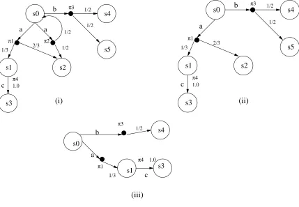
Fig.2.1 shows a simple PNS, which we use as a running example for this chapter, whereS ={s0, s1, s2, s3, s4, s5} and ∆ ={(s0, a, π1),(s0, a, π2),(s0, b, π3),(s1, c, π4)}

When an action a is requested of the system, the system responds, on its own accord, by following one of theaactions possible from the current state. Once sucha tran-sition (s, a, π) is selected the next state reached is dictated by the probability distribution

π1 π2

π3

1.0

1/3 2/3 1/2

a a _1/2

1/2 1/2 s4 s0 s1 s3 s2 b c π4 s5 s4 1/2 π3 b s0 a π1

1/3 s1 c

s3 π4 1.0 π1 π3 1.0 1/3 2/3 a 1/2 1/2 s4 s0 s1 s3 s2 b c π4 s5 (i) (ii) (iii)

Figure 2.1: (i)A simple PNS (ii)A schedule for PNS (iii)An observation for schedule

Most of the known models of computation for non-determinism and probabilis-tic choice are subclasses of PNS. These include PTS which are determinisprobabilis-tic, LTS which have no probabilistic choice, and Concurrent Markov chains which have no external non-determinism. Formally, we have:

Definition 2.1.3. A PNSP = (S,∆, sinit) is said to be aPTS provided for eachs∈S and

each a∈Act there is at most one distribution π such that s→a π.

A PNS is a labeled transition system (LTS) provided all distributions are Dirac. A PNS reduces to a Concurrent Markov chain when |Act|= 1. Finally, a PTS is a Markov chain if it is a PTS and |Act|= 1.

sched-uler is a generalization of scheduler which takes the requested action into account while resolving the non-determinism. There can be various kinds of reactive schedulers, for exam-ple deterministic schedulers which at a given state and action label, always pick the same probability distribution, policy basedschedulers which resolve the non-determinism as per pre-defined decision policies orrandomized schedulerswhich resolve the nondeterminism us-ing a random probability distribution. In this thesis we focus on randomized schedulers, and to this end we define the notion of combined transitionof PNS that takes into account the randomized schedulers, by considering all possible linear combinations. For the following definitions we fix a PNS P = (S,∆, I, sinit).

Definition 2.1.4. A combined transitionis a triple (s, a, π) where π is a convex combina-tion ofatransitions enabled froms. Formallyπ =P

t=(s,a,πt)∈∆λt·πtwhere

P

t=(s,a,πt)∈∆λt =

1.

For the simple PNS of fig. 2.1, a combined atransition froms0 is 1/2π1+ 1/2π2. Based on the notion of combined transition we will now define the notion of a path that a system might take:

Definition 2.1.5. A path σ starting from a state s0 is a possibly infinite sequence of the form s0 a0−→,π0,r0 s1. . .

an−1,πn−1,rn−1

−→ sn. . ., where for all i ≥ 0 the triple (si, ai, πi) is a

combined transition and πi(si+1) =ri.

Given a path σ letfst(σ) =s0 denote the first state, and if σ is finite, letlst(σ)be the last state of the path. We will use sa,π,r−→ σ to denote a path starting at sfollowed by σ

provided(s, a, π) is a combined transition andπ(fst(σ)) =r. Similarly, σ a,π,r−→ sdenotes an extension of path σ. Iffst(σ0) =lst(σ), the concatenation of two paths is denoted as σ.σ0. Pathσ0 _{is a prefix ofσ, denoted byσ}0 _{≤σ, if there exists a pathσ}00 _{such thatσ =σ}0_.σ00_{. Let}

For the simple PNS, {s0

a,π1,1/3

−→ s1 c,π−→4,1.0s3, s0

a,π2,1/2

−→ s0

aπ2,1/2

−→ . . .} are maximal paths. Sets of paths, under certain conditions, denote trees that can be looked upon as reactive schedules. We will first define a tree as a set of paths that identify it. Formally, we have:

Definition 2.1.6. A set of s0-rooted maximal pathsT ⊆P(s0) is said to be a tree provided it is deterministic: Ifσ a,π−→1,r1 s1 andσ

a,π2,r2

−→ s2 are inT thenπ1 =π2. Defineroot(T) =s0. We extend the transition notation to trees, i.e. T a,π,r−→ T0 _{if there is a s}

0

a,π,r

−→ sin

T and T0 ={σ ∈P_{(s) |s0} a,π,r_{−→ σ ∈T}. IfT} a,π,r_{−→ T}0 _thenT0 _{is a subtree ofT. A tree T is}

maximal provided there is no other treeT0 such thatT ⊆T0. For our running example, {s0

a,π1,1/3

−→ s1 c,π−→4,1.0 s3, s0

a,π1,2/3

−→ s2, } is a tree.

{s0

a,π1,1/3

−→ s1 c,π−→4,1.0 s3, s0

a,π1,2/3

−→ s2, s0

b,π3,1/2

−→ s4, s0

b,π3,1/2

−→ s5} is a maximal tree, and a schedule. (see definition below).

Definition 2.1.7. A s0-rooted reactive schedule is a maximal s0-rooted tree. Let Ms0 be the set of all maximal trees and, thus reactive schedules withs0 as its root.

Given a schedule T, which has resolved all non-determinism from the PNSP, we can consider sets of paths that resolve all probabilistic choice [14].

Definition 2.1.8. Given a scheduleT, a set of finite pathso is anobservation ofT if and only if:

1. for each p∈o, there existsp0∈T such thatp is a prefix of p0, and 2. if σa,π,r−→s and σa,π,r−→0s0 _{are in o, then r=r}0 _ands=s0_.

{s0

a,π1,1/3

−→ s1c,π−→4,1.0s3, s0

b,π3,1/2

−→ s4}, is an observation for the schedule,{s0

a,π1,1/3

−→

s1

c,π4,1.0

−→ s3, s0

a,π1,2/3

−→ s2, s0

b,π3,1/2

−→ s4, s0

b,π3,1/2

−→ s5}(fig 2.1),

2.1.1 Measure space

To build a measure space for a reactive scheduleT we can start with observationso

and build basic cylindrical sets out of them asBo ={σ ∈T | ∃σ0 ∈o.σ0 ≤σ}. The measure

of such a basic cylindrical set would be the product of the probabilistic choices in o, and will be denoted as mT(o). The smallest Borel field containing such basic cylindrical sets

would then form the required probability space. These constructions are rather standard and can be found in [14].

Chapter 3

Extended Generalized Probabilistic

Logic

The specification logic is required to be expressive enough to capture the properties of interest in a particular class of systems. The PNS allows us to model non-determinism along with the probabilistic choices. The behavior of PNS is determined by the schedules and their observations. Thus the first requirement of any specification logic for PNS is that it should be able to quantify over schedules. In the presence of multiple probability distributions for a given state and action label it is impossible to talk in terms of exact probabilities of properties. Therefore, the second requirement for the logic is that it should allow us to express range of probabilities for satisfying the property. We should be able to specify properties like there exists a scheduler such that P r(s|=φ) ∈[α, β] where [α, β]⊆

3.1

Syntax of EGPL

The syntax for extended GPL (EGPL) is given by the following BNF-like grammar.

ψ ::= haiψ |[a]ψ |ψ1∧ψ2 |ψ1∨ψ2 |µx.ψ |νx.ψ|φ |X

φ ::= EYψ |AYψ |φ1∧φ2 |φ1∨φ2 |A| ¬A whereY ⊆[0,1] and A∈P rop

The formulas generated from nonterminalφare referred to asstateformulas andψgenerate formulas as path formulas. The operators µ and ν bind the variables in the usual sense, and one may define the standard notion of free and bound variables. Also, we refer to an occurrence of a bound variable X in a formula as a µ-occurrence if the closest enclosing binding operator forX is µand as a ν-occurrence otherwise. The following restrictions on GPL formulas are applied to the EGPL formulas:

• in the formulaEYψorAYψ the formulaψ can not contain any free variables, and

• no sub-formula of the formµX.ψ(νX.ψ) may contain a freeν-occurrence(µ-occurrence) of a variable. In other words the formula must be alternation free.

3.2

Semantics of EGPL

The semantics of EGPL is described in terms of observations of schedules. There-fore, it is necessary to have quantifiers over schedules while talking about the properties of PNS. E is the existential quantification over the schedules and the specificationEYψ is

satisfied if there exists a schedule of the PNS which satisfies the formulaψ with probability which is in the interval Y. AY formulas quantify over all schedulers and the PNS satisfies

aAformula if all the schedules of the system satisfy the formula with probability inY. An observation rooted atssatisfies a state formula if ssatisfies the formula. The path formu-las when interpreted against a schedule have a measurable set of observations that satisfy them. That is why they are also referred to asfuzzy formulas[14]. An observation satisfies thehaiψ if the uniquea-successor satisfies ψ. In order to formally specify the semantics of EGPL we define two mutually recursive functions as follows.

• Θs: Ψ×Ms→Os, which returns the set of observations of a schedule, T ∈Ms, that

• |=⊆S×Φ which indicates whether a state formula is true at a states∈S. Fix a PNS P = (S,∆, I, s0), and fix a states∈S.

Definition 3.2.1. The function Θs(ψ, T) is ∅ if root(T) 6= s. Thus, assuming that

root(T) =swe have Θs(haiψ, T) ={o∈OT | o

a,π,r

−→o0_∧T a,π,r_−→T0_∧o0 _∈Θ

root_(T0₎(ψ, T0)} Θs([a]ψ, T) ={o∈OT |(o

a,π,r

−→o0) ⇒(T a,π,r−→ T0∧o0 ∈Θroot_(T0₎(ψ, T0))} Θs(ψ1∧ψ2, T) = Θs(ψ1, T)∩Θs(ψ2, T)

Θs(ψ1∨ψ2, T) = Θs(ψ1, T)∪Θs(ψ2, T) Θs(X) = Θs(ψ) where X7→ψ

Θs(µX.ψ) =Sinf_i=0Mi, where M0=∅ andMi+1= Θs(ψ[X7→Mi], T)

Θs(νX.ψ) =Sinfi=0Ni, where N0=OT andNi+1 = Θs(ψ[X 7→Ni], T)

Θs(φ, T) =

      

OT ifs|=φ

∅ otherwise

Once a schedule, T, resolves all the non-determinism in the PNS, the systems be-have like a PTS, hence the following theorem follows directly from the result of measurability of Θs in [14].

Theorem 1. For any given scheduleT, s∈S andψ∈Ψ, Θs(ψ, T) is measurable.

s|=AYψ iff ∀T ∈Ms, mT(Θs(ψ, T))∈Y

s|=EYψ iff ∃T ∈Ms, mT(Θs(ψ, T))∈Y

s|=φ1∧φ2 iffs|=φ1 and s|=φ2

s|=φ1∨φ2 iffs|=φ1 or s|=φ2

s|=A iff A∈I(s)

s|=¬A iff A6∈I(s)

1.0

1/2

1/2

1.0

1.0

1/2

1/2

s2’

s4

s3

s1

s2

λ2

λ1

π1

π2

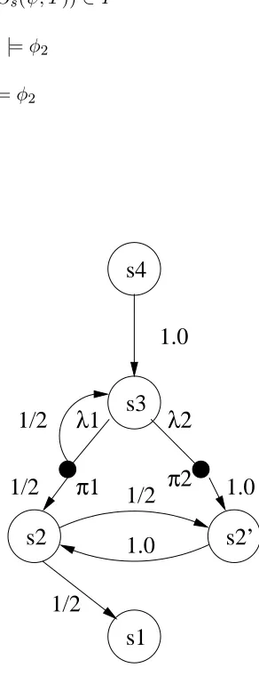
Figure 3.1: PNS for token stabilization algorithm

a dummy action label a to the system, and define that all the transitions are made on a. From [5],ψ=µX.((s1)∨ haiX) represents theeventually stabilizeproperty. φ=A_[1.0,1.0]ψ

specifies that for all the schedulers the probability of satisfyingψis 1.0. φgives the required specification.

Chapter 4

Model Checking of PNS

The PNS allows to model the non-determinism and EGPL gives the specification which ranges over schedulers. The quantitative analysis of EGPL formula with respect to PNS, is essentially the computation of minimum(or maximum) probabilities of satisfying the formula over the set of schedulers. We intend to compute results of the formP r(s0, ψ)∈[l, u] where [l, u] ⊆ [0,1]. In [14], Cleaveland et. al. propose an algorithm modchk-fuzzy, for model checking GPL properties with respect to a PTS. The algorithm generates a product graph from the PTS andFisher-Ladner closureof the GPL formula. A system of equations is generated from the product graph and one of the solutions of the equations gives the measure of the GPL formula for the PTS. A PNS and a PTS differ only in the transition probabilities where a PTS has a single probability associated with every transition, a PNS has a range of probability values corresponding to the various possible schedules of the PNS. This observation forms the basis of extending the algorithm for quantitative analysis of PNS. In the following sections we tailor the algorithm modchk-fuzzy to compute the probabilities for a restricted subset of EGPL properties with respect to PNS.

4.1

Outline of the approach

• FromL, s0, T, ψ construct a dependency graph

• From the dependency graph extract a set of constraints

• Minimize(maximize) the root variable with respect to constraints.

Before going into details of each step, two important comments are in order.

• The presence of multiple probability distributions in PNS, makes it impossible to talk in terms of exact probabilities of properties. Therefore, we are interested in computing the minimum and maximum probabilities of satisfying the property, where the minimum and maximum are computed over all possible schedules. A randomized schedule is uniquely identified by the random probability with which it resolves the non-deterministic choices, i.e., the set of values it assigns to the λi’s(refer definition

2.1.7,2.1.4 ). These λi’s specify the constraints over transition probabilities. So a

maximization(minimization) of the root node of dependency graph subject to the constraints gives the schedule corresponding to the maximum(minimum) probability of satisfying the property. Thus the schedule,T, refers to the unknown schedule which gives the maximum(minimum) probability of satisfying the property. In the following discussion we assume the existence of such an optimal scheduleT.

• We use EGPL without recursion for the specification of properties. The reason for the restriction is explained towards the end of the chapter. In the rest of the chapter EGPL refers to the restricted set of properties given by:

ψ ::= haiψ|[a]ψ |ψ1∧ψ2 |ψ1∨ψ2 |φ|X

φ ::= EYψ |AYψ |φ1∧φ2 |φ1∨φ2 |A | ¬A whereY ⊆[0,1] and A∈P rop

4.2

Graph Construction

Fix a state s0 and a fuzzy(path) formula ψ. The first step in modchk−f uzzy involves constructing a graphP G(s0, ψ) that describes the relationship between the quantity

mT(Θs0(ψ, T)), that we wish to compute, and the quantities of the form mT0(Θs(ψ, T0)), wheresis a state reachable froms0 andψ0is an (appropriate) sub-formula ofψ. This graph has vertices of the form (s, F), wheres∈S andF is a set of fuzzy formula, The edges from (s, F) then provide “local” information regarding m_T(Θs(ψ, T)).

Definition 4.2.1. For a closed fuzzy formulaψdefine the (Fisher-Ladner) closure, written as Cl(ψ), as the smallest set of formula satisfying the following rules:

• ψ∈Cl(ψ)

• If ψ0 ∈Cl(ψ) then

– if ψ0 =ψ1∧ψ2 or ψ1∨ψ2 then ψ1, ψ2 ∈Cl(ψ)

– if ψ0 =haiψ00 or [a]ψ00 for some a∈Act, then ψ00∈Cl(ψ)

One may easily show that Cl(ψ) contains no more elements than ψ contains sub formula.

The node set N in the graph is a subset of the set S ×2Cl(ψ); that is, nodes have form (s, F), where s∈S and F ⊆Cl(ψ). A node is classified according to the first rule, among the following, that it satisfies.

• (s, F) is anempty nodeifF =∅.

• (s, F) is afalse nodeif there exists a state formulaφ∈F withs6|=φor if there exists a formula of the formhaiψ0 and there is no s0 such thats→a s0.

• (s, F) is a true node if (a)it has at least one state formula φ∈F such that s|=φ or (b) it has at least one [a]ψ ∈ F but there are no transitions of the form s →a s0 for any s∈S.

• (s, F) is anand node if there exists a formulaψ1∧ψ2 ∈F

• (s, F) is anor nodeif there exists a formula ψ1∨ψ2∈F

• (s, F) is anaction node if every formula inF has the formhaiψ0 or [a]ψ0

The edges in the graph are labeled by the elements drawn from the set Act∪ {²+, ²−}

(assuming²+, ²−∈/Act). Define the set of action labels in a set of formulaF asaction(F) =

{a∈Act|∃ψ.haiψ∈F∨[a]ψ∈F}. The edge set E ⊆N ×(Act∪ {²+, ²−})×N is defined as follows.

• else if (s, F) contains state formulas then (s, F), ²+,(s, F))∈ E, where F0 isF with all the state formulas deleted.

• else ifψ=ψ1∧ψ2∈F then ((s, F), ²+,(s, F − {ψ} ∪ {ψ1, ψ2}))∈E)

• else ifψ=ψ1∨ψ2 ∈F then ((s, F), ²+, F − {ψ} ∪ {ψ1})∈E, ((s, F), ²+, F − {ψ} ∪

{ψ2})∈E, and ((s, F), ²−,(s, F − {ψ} ∪ {ψ1, ψ2}))∈E);

• else if (s, F) is an action node, let Fa={ψ0|haiψ0 ∈F or[a]ψ0 ∈F}. Then for any a∈

ActwithFa6=∅ands0 ∈Ssuch that∃π.(s, a, π)∈∆∧π(s0)>0,((s, F), a,(s0, Fa))∈

E.

The graph construction is guaranteed to terminate; this is due to the fact that all the formulas in the construction are in Fisher-Ladner closure ofψ [9].

The edges in the graph indicate a “local relationship” between its end nodes. To see this, first note that if (s, F) is false then [[(s, F)]] =∅andmT(Θs(F, T)) = 0 and if it is an

empty node then all observations of scheduleT satisfy the formulaF i.e.[[(s, F)]] =OT and

mT(Θs(F, T) = 1. If the node is anor nodei.e. F =F0∪{ψ1∨ψ2}then the semantics of the logic entails that∧F and (∧F0∧ψ1)∨(∧F0∧ψ2) are logically equivalent. Therefore we have

mT(Θs(F, T)) =mT(Θs(∧F0∧ψ1, T)) +mT(Θs(∧F0∧ψ2, T))−mT(Θs(∧(F0∪ {ψ1, ψ2}), T)) This observation is encoded in ²+, ²− edges emanating from the or node. Similar obser-vations can be made for other nodes except the action nodes. Under the assumption of existence of optimal schedule T the PNS reduces to PTS and we have the following results from [14], which relate the nodes to their measures.

Lemma 1. For the product graph P G(s0, ψ) = (N, E)

• If (s, F) is an empty node then

m_T([[s, F]]) = 1

• If (s, F) is a false node then

• If(s, F)is an or-node with edges((s, F), ²+,(s, F1)),(((s, F), ²+,(s, F2))and(s, F), ²−,(s, F3)) then

m_T([[(s, F)]]) =m_T([[(s, F1)]]) +mT([[(s, F2)]])−mT([[(s, F3)]])

• If(s, F)is an action node thenmT([[(s, F)]]) = Q a∈action(F)

P ((s,F),a,(s0_,F0_))∈E

P r(s, a, s0)×

m_T([[(s0, F0)]])

• If (s, F) is any other node then it has a unique successor (s, F0)

m_T([[(s, F)]]) =m_T([[(s, F0)]])

4.3

Generating constraints from the graph

We give a method to generate a set of constraints from the graph. The constraints have one variable for each node of the graph. For every variable there is exactly one equation with the variable on the LHS. The transition probabilities are expressed as variables whose values are given by the values of λi’s and corresponding probability distributions πi. For

example,(refer Fig. 3.1), P r(s3, a, s2) = y(s3,a,s2) = λ1 ∗ 1

2 +λ2∗0. The constraints are generated according to following rules.

1. Ifn is aempty node then Xn= 1;

2. Ifn is a false node thenXn= 0;

3. If there is an edge of the form (n, ²+, n0) then the equations for Xn is

Xn=

X (n,²+_,n0_)∈E

Xn0 − X (n,²−_,n0_)∈E

Xn0 4. Ifn= (s, F) is an action node, let An={a|(n, a, n0)∈E}. Then,

Y

a∈An

X (n,a,(s0_,F0_))∈E

(ys,a,s0·X_(s0_,F0₎) where ∀a ∈ An.∀s0 ∈ S. ys,a,s0 = P

iλis,a ∗πis,a(s0) whereπs,ai are the probability

distributions fromson aand P

The action node makes a transition with the probability defined by the scheduler. The λi’s correspond to the unknown scheduler, T, which gives the maximum(minimum)

value. The product part of the action node equation comes from the fact that transition with different action labels are independent of each other. Maximizing(minimizing) the root variable with respect to the constraints gives the maximum(minimum) measure over all possible schedules. Note that we use the optimization only for the root variable, that is we compute the minimum(maximum) value of satisfying the property starting at the root state. The probability values for internal nodes correspond to the schedule which minimizes(maximizes) the root node, and hence are not necessarily optimal for the corre-sponding node and sub formula pair.

Under the assumption of existence of the optimal schedule, T, the PNS becomes a PTS and the following lemma follows from Lemma 1.(refer Lemma 19 in [14])

Lemma 2. Let Υ={Xn = Υn} be the set of equations generated above, and let measure

values corresponding to optimal schedule T be V = {Xn = mT(Θs(∧F, T)}, where n =

(s, F). Then V is a solution to Υ.

4.4

Model Checking Example

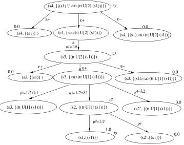
We illustrate the model checking algorithm for PNS of fig.3.1 and the property

φ=E_[0.25,1.0](ttU[3] (s1)), whereU[k] is the bounded until property defined as

φ1U[0]φ2 =φ2

φ1U[k]φ2 =φ2∨(φ1∧ hai(φ1U[k−1]φ2))

The property specifies that there exists a schedule so that probability of reaching state (s1) in 3 or less steps is at least 0.5. It suffices to check if the maximum probability is greater than equal to 0.25. The product graph is shown in fig.4.1. The root node is an or node and one of the disjuncts is a false node as s4 6|= (s1). So node (s4,{hai(tt U[2] (s1))}) is the only node to explore. Note that the nodess0

2 ands3 can not reachs1 in one step hence they are denoted as false nodes. Constructing the product graph in a similar fashion we get the following set of constraints to maximize the root variable.

MAXx4;

(s4, {(s1)} )

(s4, {((s1) \/ <a>(tt U[2] (s1)))})

(s4, {<a>(tt U[2] (s1))})

(s4, {(s1),<a>(tt U[2] (s1))})

(s3, {(tt U[2] (s1))})

1/2∗λ1

y2= y3=1/2∗λ1 y4=λ2

x3 ε+ ε+ ε− a 0.0 0.0 x4 ε+ ε+ ε− 0.0

(s3, {(s1)} ) (s3, {<a>(tt U[1] (s1))}) _{(s3, {(s1),<a>(tt U[1] (s1))})}

0.0

(s3, {(tt U[1] (s1))}) (s2, {(tt U[1] (s1))}) _{(s2’, {(tt U[1] (s1))})}

0.0 (s1,{(s1)}) 1.0 y5=1/2 x2 x1 (s2’,{(s1)}) y6 0.0 y1=1.0

Figure 4.1: Product graph

x3=y2∗0+y3∗x2+y4∗0;y3=λ1/2

whereλ1+λ2= 1.0

x2=y5∗x1+y6∗0;y5 =1/2

x1=1.0

The maximum value ofx4 = 0.25 is obtained for the scheduler which assignsλ1 = 1.0, λ2= 0.

The complexity of the product graph construction is linear with respect to the size of the product set of states of PNS and the Fisher-Ladner closure of the specification i.e.

Model checking the complete EGPL logic with fix points cannot be done using the above method based on product graph. The quantitative analysis of µ and ν properties requires computation of maximum(minimum) for a set of variables corresponding to the strongly connected components in the product graph(refer [14]). The back substitution of these maximum(minimum) values does not ensure the optimal probability measures for the nodes dependent on the variables of strongly connected component.

Chapter 5

Implementation and Case Studies

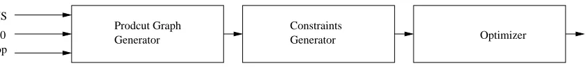
Constraints Generator Prodcut Graph

Generator s0

PNS

prop

Optimizer

Figure 5.1: Quantitative Model Checker

5.1

Quantitative Model Checker

The model checker has three components as seen in Fig.5.1. The product graph generator, takes a PNS model, a start states0and a path property of PNS, and generates the product graph of Fisher-Ladner closure of the property and the PNS. This product graph is used by the constraint generator which generates a set of constraints, and the optimizer maximizes(minimizes) the variable corresponding to the root node of product graph with respect to these constraints. The PNS is described using a PRISM[10] like language (see appendix A for sample input file). States are uniquely identified by the set of atomic propositions they satisfy and they are hashed to positive integers. Transitions are identified with the start state, next state action label and probability interval. A typical transition input looks like: []s=0 ->[a] 0.5:s=1 + 0.5:s=0 , whereais the action label. The non-determinism in the PNS is specified by allowing the model to have multiple lines where a given state on a given label goes to different probability distributions. The parser generates an interval graph from the input PNS which is used by the product graph generator. The key wordCOMPUTEprovides the start state and the path property to be analyzed. We use the optimization tool LINGO1 to solve the non-linear optimization and generate the probability measure. In the next section we present the modeling and quantitative analysis of the token based randomized self-stabilization protocol.

5.2

Randomized Self-Stabilizing Protocol(RSSP)

The protocol we consider in this section is due to Israeli and Jalofan [8]. It is a token based protocol used by a system of n processes connected in an oriented ring and having bidirectional communication. The goal of the protocol is to reach the ”stable” state

1110 1101 1011 1111

0111

GOOD

1100 0011 0101 1010 0110 1001

1

2

3 4

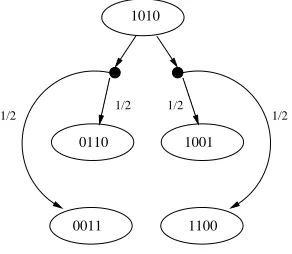
Figure 5.2: PNS for 4 processes token based randomized self-stabilization protocol

1010 1100 0011 0110 1001 1/2

1/2 1/2 1/2

Figure 5.3: A typical execution step in the protocol

starting from an ”illegal” state. Stable state is the one where exactly one process has the token and an illegal state is the one where more than one processes have token. The processes having the token are called active processes. The scheduler randomly picks one of the active processes and this process propagates the token towards its left or right with equal probability. When a processes has more than one token the tokens are merged into a single token.

(0011), or with 1/2 the probability it goes to state (0110). Similar execution can be seen for the choice of process 3 in fig.5.3

It is easy to see that the size of the graph is exponential in the number of processes,

O(2n_{). Therefore, even a small model of such system would generate large of number states}

in the product graph which will proportionately generate large number of constraints and variables. We focus on systems with 4 and 5 processes and exploit symmetry to reduce the number of states while preserving the quantitative behavior of the system.

5.2.1 Abstraction based model

The evolution of RSSP from a particular state depends on the neighborhood struc-ture of each process. By neighborhood strucstruc-ture we mean whether the process has active or inactive process to its left and right.2

• If an active process has an active process on its left and right then the system evolves to a state with one less number of tokens with probability 1.

• If it is adjacent to one active and one inactive process then with half probability it evolves to one less number of tokens and half probability it goes to state with the same number of tokens.

• If both its neighbors are inactive then with probability 1 it goes to a state with same number of tokens.

So the first requirement of an abstraction for RSSP is that the set of states grouped together must have same number of tokens The second requirement is that they should have the same neighborhood structure for all the component processes. The abstraction described in the section is based on the observation that ifnprocesses are arranged in an oriented ring where

mare active andn−mare inactive then, finite number of rotations of the processes merely relabels the processes while preserving their neighborhood structures. The finite number of rotations refers to the bijective function which relabels the active(inactive) processes of one state to the active(inactive) processes of another state while preserving the neighborhood structure.

1 2 3 4 1 2 3 4 1 2 3 4 1 2 3 4 (a) t3

1 1 1

1 1 1

1 1 1 0 0 1 1 0 0 1 s’ s" s 1 2 3 4 1 2 3 4 1 2 3 4 1 2 3 4 1 2 3 4 1 2 3 4 (b) t21 1 1 1

1 1 1

0 0 0 0 0 0 0 0 1 1 (c) 1 1 1 1 0 0 0 0 t22

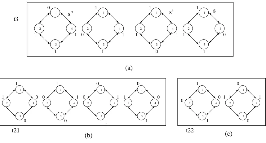
Figure 5.4: Equivalent states of 4 process PNS

Consider the 4 process PNS for RSSP, the state space can be partitioned into four disjoint subsets,{t4, t3, t2, t1}, whereticorresponds to the state havingitokens (see fig.5.4).

There are¡₄

i

¢

states corresponding toti fori= 1 to 4. There are 4 states where system can

have 3 tokens and 6 states where the system has 2 tokens. We claim that all the 4 states of

t3 are identical with respect to qualitative properties. To see this note that all the 4 states can be obtained by rotation of each other. For example consider state s = (1,1,1,0), a rotation takes the state tos0 = (1,1,0,1) or s” = (0,1,1,1), depending on the direction of rotation (fig.5.4). Ins, processp3has the token and is adjacent to processp4on right which doesn’t have the token and process p2 on left which has the token. Similar configuration can be seen for processp2 ins0 _{and processp4 ins”. So an execution of PNS which chooses}

p3 inscan be simulated by choice ofp2(p4) in s0(s”). Similar mappings can be established forp1, p2 andp4. Hence all the states int3 are identical with respect to qualitative behavior of the system. However, subset t2 has to be partitioned into subsets t21 and t22, because elements in t21 cannot be obtained by finite rotation of elements in t22 and vice versa. So, we have the following partition of state spaceP(S) ={t4,t3,t21,t22,t1}. The following

Theorem 2. Consider the relation, R, induced by the partition, P(S),sRs0 iffs, s0 ∈ti. R

is a probabilistic bi-simulation.

Proof. • R is an equivalence relation.

• LetsRs0_{. The transition probability,P r(s, a, r) =}P

iλiP r(pi, a, r) where 1≤i≤4 is

the number of active processes ins. The same transition probability can be obtained froms0 asP r(s, a, r0) =λ1∗P r(B(p1), a, r) +λ2∗P r(B(p2), a, r) +λ3∗P r(B(p3), a, r). where rRr0 _{and B is the bijective function corresponding to finite rotation which}

relabels the processes ins to processes ins0.

5.2.2 Experimental Results

t1 t5

t4

t22 t21

t31 t32

1

1

1/2 1/2 1/2

1/2

1.0

1/2

1/2 1.0

1.0 1/2

1/2

s2’ s4

s3

s1 s2

(a) (b)

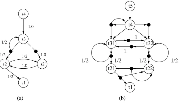
Figure 5.5: Abstract model of RSSP (a) 4 process system (b)5 process system

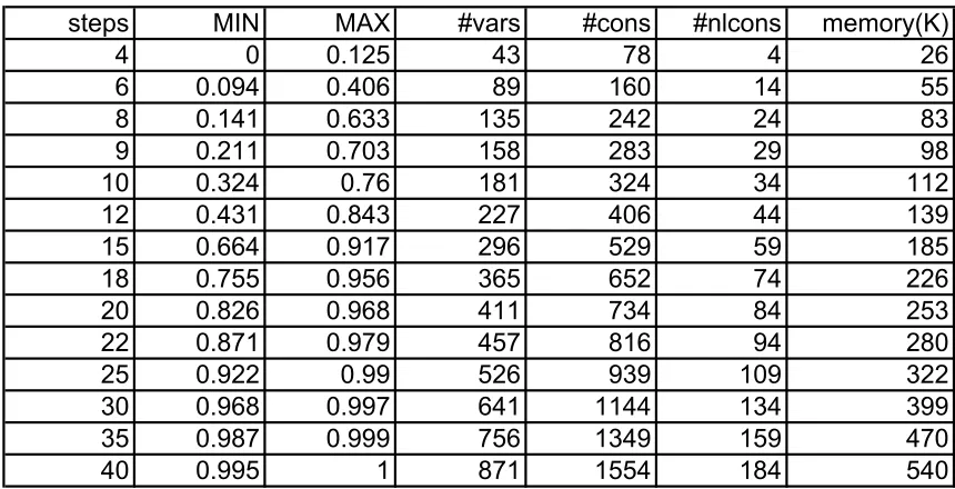
Each step corresponds to the scheduler randomly picking up an active processes and the process then passing the token to its left or right with equal probability. The property is specified using the bounded until operator as follows

(ttUx(t1 =1))

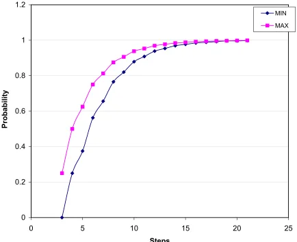
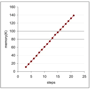
Table 5.1 gives the minimum(MIN) and maximum(MAX) probability of reaching the stable state inxsteps. An interesting property to note from Table 5.1 is that the minimum (max-imum) probabilities of satisfying the bounded until properties under randomized schedulers is the same as minimum(maximum) probabilities obtained by considering non-deterministic schedulers[3]. This stands as a witness to the theorem in [2], which states that for bounded until properties it is sufficient to minimize or maximize over the non-deterministic schedules. The number of variables and constraints grow linearly with respect to the number of steps (see fig5.9). This is expected since the number of nodes in the product graph varies linearly with the closure of formula, which keeps increasing with steps, if the system is kept constant (refer chapter 4). The memory usage of LINGO varies linearly with the number of constraints and variables(see fig5.7). The system has been optimized to reduce the number of redundant equations of the form xi=xj and xi=0. This optimization is possible in the

absence of recursion as every node(variable) of the product graph is referred exactly once in the LHS and exactly once in the RHS of the constraints. The non-linear constraints correspond to the randomized scheduling at state t3. The number of nodes corresponding tot3 in the product graph, increase linearly with the number of steps and hence the number of non-linear constraints also increase linearly.

!

!

! !

! ! !

! !

! ! !

! !

! !! ! !

! ! !

! !!

! !!

!! !! !

! !! ! !! !

!! !!

!! ! !!! !

Table 5.1: Quantitative Analysis of RSSP for 4 process system

! !

! ! !

!

! ! ! !

! !

! ! !

! !! ! ! !

! !! !!

! !!! ! !

!!

Figure 5.8: Minimum and maximum probabilities of stabilizing in x steps for 5 process RSSP

Chapter 6

Compositional Verification of PNS

The study of compositionality is an essential component of top-down design method-ology. In this approach we wish to decompose the specification of a composite system into sufficient and necessary specifications of the components of a system. Consider a com-posite system P4X, where 4 is a process algebra operator and X is the system is to be designed(say X). Let F be the required specification for the composite system. We wish to compute individual sub-specifications FX, for the unknown component such that the

following is satisfied.

X |=FX ⇔P4X |=F

Clearly, while maintaining soundness we want the specificationFXto be as weak as possible

so that we have greater latitude with possible implementation of X. In [12], Larsen et.al. proposed a decomposition scheme for extended PML formula and SCCS like algebra for PTS. In this work we develop a similar calculus CN P P, and add a non-deterministic composition operator for the PNS composition. We then define the decomposition operator

W_{4 which gives the sub specification for the unknown component. In the end we prove a}

6.1

Calculus for PNS

Definition 6.1.1. Let Act be a set of actions. Then the calculus of non-deterministic probabilistic processes (CNPP) over a given set of actions Act has the following syntax

P ::=0|a.P|P ⊕Q|P ⊕µQ|P ×Q

In the above definition 0 denotes completely inactive process, whereas a.P can perform the actionaand then behave likeP. The processP×Qcan only make a transition

c = (a, b) when both the components P and Q perform their corresponding actions. The probabilistic summation constructP⊕µQ, selects the processP(Q) with probabilityµ(1−µ)

if bothP and Qhave transition on the action labela, else it selects the process having the transition on awith probability 1. If neither of the processes has a transition on athen it selects neither of them. The non-deterministic summation operator P ⊕Q selects P with probability λ ∈ [0,1] and Q with probability 1−λ if both have transitions on action a, otherwise the behavior is same as probabilistic summation.

Definition 6.1.2. Let Act be a set of actions. In the presence of action based non-deterministic choices we cannot calculate the exact probabilities, therefore we define the

transition probabilities in terms of intervals in[0,1]. Let N P r be the set of processes. The transition probability intervals π are defined as follows:

π(0, a, P) = [0,0] for alla∈Actand forP ∈N P r π(a.P, b, Q) =

  

[1,1] ifP =Q, b=a

[0,0] otherwise

π(P ×Q,ha,a¯i, P0×Q0) =                   

[l, u] where l=lp∗lq,

u=up∗uq,

[lp, up] =π(P, a, P0),

[lq, uq] =π(Q,a, Q¯ 0]

π(P ⊕Q, a, R) =                               

[l, u] where l=min(lp, lq),

u=max(up, uq),

[lp, up] =π(P, a, R),

[lq, uq] =π(Q, a, R) ifP →a, Q→a

[lp, up] ifQ6→a

[lq, uq] ifP 6→a

[0,0] otherwise

π(P ⊕µQ, a, R) =

                  

[µlp+ (1−µ)lq, µup+ (1−µ)uq] where [lp, up] =π(P, a, R),

[lq, uq] =π(Q, a, R) ifP →a, Q→a

[lp, up] ifQ6→a

[lq, uq] ifP 6→a

[0,0] otherwise

For π(P, a, P0) = [l, u], definemin(max)π(P, a, P0) =l(u). For the non-deterministic sum-mation operator, the probabilityπ(P⊕Q, a, R) = [l, u] wherelis the minimum anduis the maximum of the two probabilitiesπ(P, a, R) andπ(Q, a, R), which corresponds to combined transition of the PNS where the next state transition probabilities are defined by the convex combination of available probability distributions.

In the next section we define a variant of extended PML([12]) which is used as the specification logic.

6.2

A variant of extended PML

Syntax of the logic is given as follows

F ::=tt|c|F∧G|¬F|[hai[x1,y1]F1, ...,hai[xk,yk]Fkwhere φ(x,y)]|σc.F whereσ={µ, ν}

The logic essentially puts constraints on the minimum and maximum transition probabilities at each step. These constraints, as we will see, define the intervals of transition for the unknown system. Semantics of the logic is given with respect to the set of probabilistic non-deterministic processes N P r.

• [[tt]] =N P r

• [[σc.F]] = [[F]] where [σc.F/c]

• [[F∧G]] = [[F]]∩[[G]]

• J[hai[x1,y1]F1, ...,hai[xk,yk]Fkwhere φ(x1, y1, . . . , xk, yk)]K

={P ∈V| φ(min{π(P, a,[[F1]])}/x1, max{π(P, a,[[F1]])}/y1, . . . ,

min{π(P, a,[[Fk]])}/xk, max{π(P, a,[[Fk]])}/yk)}

We now have the framework to answer the following question.

Given a PNSP, an unknown PNSX, and the composition operator4 ∈ {a., P⊕µ, P⊕, P×},

computeW_{4(F) such that 4X |=F iff X|=}W_4(F)

6.3

Decomposing Formulas

Definition 6.3.1. Leta∈Act,µ∈]0,1[, andP a process. We define the transformersW₄

inductively as follows:

W_{4(tt) =tt}

W_{4(c) =}W_{4(F)where[c7→F]} W_{4(σc.F) =}W_{4(F)[c7→σc.F]} W_{4(F ∧G) =}W_4(F)∧W_4(G)

W_{4(¬F) =¬}W_4(F)

W_{b.(F) =}                         

tt ;b6=a, φ(0,0) ff ;b6=a,¬φ(0,0)

ff ;b=a,Γ ={}

W

ν∈Γ ( V

νi=1

Fi∧ V νi=0

¬Fi) ;otherwise

where Γ denotes the set of tuples ν = (ν1, . . . , νn) where each νi = xi =yi = 0 or 1 such

thatφ(x,y) holds.

W_P⊕

µ(F) =

              

F ;P 6→a

¬< a >_[0,1]tt∨GP,F ;P →a andP |=F

GP,F ;P →a andP 6|=F

where GP,F = [< a >[x1,y1] F1, ..., < a >[xn,yn] Fn where φ(. . . ,(µ∗min{π(P, a,[[Fi]])}+

(1−µ)∗xi)/xi, . . . ,(µ∗max{π(P, a,[[Fi]])}+ (1−µ)∗yi)/yi, . . .)] W_{P⊕(F) =}

              

F ;P 6→a

¬< a >_[0,1]tt∨GP,F ;P →a andP |=F

GP,F ;P →a andP 6|=F

where GP,F = [< a >[x1,y1]F1, ..., < a >[xn,yn]Fnwhere

φ(. . . , min(min{π(P, a,[[Fi]])}, xi)/xi, . . . , max(max{π(P, a,[[Fi]])}, yi)/yi, . . .)]

In the following < a > denotes the ordered pair < b, c >.

W_{P×(F) =}

                

tt ;P 6→b andφ(0,0)

ff ;P 6→b and¬φ(0,0)

V 1≤i≤M,1≤j≤n

< c >_[xi,j,yi,j]W_P

i×(Fj)whereφ

0 _{holds ;P →}b

where, Pi’s are the b−derivatives of P such that, P →b

[αi,βi]

Pi and

φ0_{=φ(. . . , min}

Theorem 3.

4(X)|=F iffX |=W_4(F)

Proof. By induction on the structure of F.

• F =tt, vacuously true.

• F =c, under assumption that there are no unbounded variables, let [c7→F0]

4(X)|=c

⇔ 4(X)|=F0

⇔X|=W_4(F0_{), by ind. hyp.}

• F =¬F

4(X)|=¬F

⇔ 4(X)6|=F

⇔X6|=W_{4(F), by ind. hyp.}

⇔X|=¬W_4(F)

• F =F ∧G

4(X)|=F∧G

⇔ 4(X)|=F ∧ 4(X)|=G

⇔X|=W_{4(F)∧X |=}W_{4(G),by ind. hyp.}

⇔X|=W_4(F)∧W_4(G)

1. b.X |=F iffX|=W_b.(F).

The base cases are trivially true. Suppose thatX|= W

ν∈Γ ( V

νi=1

Fi∧ V νi=0

¬Fi) where

ν ∈ Γ is the set ofn-tuples such that νi =xi =yi = 0 or 11 and φ(x,y) holds.

Then on making the transition on b, we enter process X which models exactly those Fi such that the condition of φholds. Hence,b.X |=F.

Suppose thatb.X |=F, and letirange over the formulas such thatX|=Fiandj

range over the formulas such thatX 6|=Fj. ThenX |=V_iFi∧V_j¬Fj. Now the

conditionφdetermines the set ofFi’s andFj’s. Note that there can various such

partitions satisfying the condition φ, and the set Γ ranges over all such tuples. HenceX |=W_b.(F).

2. P ⊕X|=F iffX|=W_4(F)

If P 6→a then X has to model F, as the scheduler will always schedule X. If

P →a andP |= F then either X |= ¬ < a >_[0,1] i.e. 6→a or X |= GP,F.

Sup-pose that X |= GP,F. GP,F is the same as F except that xi is replaced by

min(min{π(P, a,JFiK)}, xi) and yi by max(max{π(P, a,JFiK)}, yi). By

defini-tion of⊕,π(P ⊕X, a,JFiK) = [li, ui] whereli =min(min{π(P, a,JFiK)}, xi) and

ui = max(max{π(P, a,JFiK)}, yi). From the supposition, φ(l,u) is true, hence

P ⊕X|=F.

Similar argument holds for the only if part.

3. P ⊕µX|=F iffX|=W4(F)

Follows from 2. 1

4. P ×X|=F iffX|=W_4(F)

If P 6→b then by definition of P ×X, there is no transition on < b, c >. So, if

φ(0,0is true thenP can be lock-step composed with anyXand the system will satisfyF. Otherwise, if φ(0,0) is false then no system X when coupled with P

would satisfy the formula. IfP →b , then suppose

X|= V 1≤i≤M,1≤j≤n

< c >_[xi,j,yi,j]W_P

i×(Fj) whereφ 0 _holds

where, Pi’s are the b−derivatives ofP such that,P →b

[αi,βi]

Pi and

φ0=φ(. . . , min

i=1 toM{αi∗xi,j}/xj, . . . , maxi=1 toM{βi∗yi,j}/yj, . . .)

By the definition of the × operator, π(P ×X, < b, c >, Pi ×[[WPi×(Fj)]]) =

[αi ∗ xi,j, βi ∗ yi,j] and by induction hypothesis, Pi ×[[WPi×Fj]] |= Fj. So

min

i=1 toM{αi∗xi,j}gives the minimum probability ofP×Xsatisfying< b, c > Fj

and byφ0 _{this minimum probability satisfies φ. Similar argument holds for the}

maximum probability. HenceP ×X |=F.

P ×X|=F

⇔Pi×X0 |=Fj for all 1≤i≤M,1≤j≤n

⇔X0|=W_P

i×(Fj) for all 1≤i≤M,1≤j≤nby ind. hyp.

⇔X|= V

1≤i≤M,1≤j≤n

< c >[xi,j,yi,j]WPi×(Fj)

π(P ×X, < b, c >, Pi×[[WPi×(Fj)]]) = [αi∗xi,j, βi∗yi,j]

∴min(π(P ×X, < b, c >,[[F_j]]) =min{α_i∗x_i,j}

∴φ⇒φ0

HenceX |=W_P×(F)

6.4

A Signal Handler Example

repair alarm

Resources

Handler

Signal

Figure 6.1: Resource and signal handler system

In order to illustrate the above decomposition scheme, we consider a system con-sisting of a signal handler and resources(Fig6.1). The resources fail with certain probability(2/3) and they generate an alarm(alarm). The signal handler on receiving the alarm can either buffer it and wait for more alarms or buffer it and switch to serving the alarms. Since the alarms are generated pretty frequently we would like the signal handler to buffer and serve more frequently rather than buffer and wait for more alarms. We model a 2 resource scenario, where process P0 denotes both the resources working and P0 |= (Good), where (Good) is a atomic proposition. P1 and P2 denote failure of 1 and 2 resources respectively.

P1 one resource is failed and the other is working, so it can either generate another alarm and go to P2, or it can remain in P1. P1 and P2 on receiving therepair signal go back to

P0. In terms of process algebra the system is described as

P0 =halarmi.P0⊕1/9(halarmi.P1⊕1/2halarmi.P2)

P1 = (halarmi.P1⊕2/3halarmi.P2)⊕ hrepairi.P0

We want the composite system of signal handler and resources to satisfy the property that an alarmsignal generated by the resources should be received by the signal handler(SH) with high probability and following it therepair signal should be generated by signal han-dler and received by resources with high probability. The composite system should revert to the state which models the proposition (Good). The property can be specified in extended PML as:

F = [halarm, alarmi[x,y](F1) whereφ(x, y) = (y > λ)] whereλis a constant in [0,1] and

F1= [hrepair, repairi[x0_,y0_](Good) where Ω(x0, y0) = (x0 = 1.0∧y0 = 1.0))]

We derive a specification forSHby using our results on compositional verification: The composite system P0×SH |=F iff SH|=WP0×(F).

1. W_P 0×(F)

=halarmi[x0,y0]WP0×(F1)∧ halarmi[x1,y1]WP1×(F1)∧ halarmi[x2,y2]WP2×(F1)

where φ0(x0, y0, x1, y1, x2, y2) = φ(max{4/9∗y1,4/9∗y2,1/9∗y0}/y) = max{4/9∗

y1,4/9∗y2,1/9∗y0}> λ), sinceP0 alarm−→

[4/9,4/9]P1, P0

alarm

−→

[4/9,4/9]P2, and P0

alarm

−→

[1/9,1/9]P0 2. W_P

0×(F1) =ffP0 6

repair

−→

3. W_P 1×(F1) =hrepairi[x0

1,y10] W_P

0×((Good)) where Ω

0_(x0

1, y01) = Ω(min{1.0∗x01}/x0, max{1.0∗y10}/y0) = (x0

1= 1.0∧y01= 1.0), sinceP1 repair−→ [1.0,1.0]P0 =hrepairi[1,1]WP0×((Good))

4. W_P 2×(F1) =hrepairi[x0

1,y10] W_P

0×((Good)) where Ω

0_(x0

1, y01) = Ω(min{1.0∗x01}/x0, max{1.0∗y10}/y0) = (x0

1= 1.0∧y01= 1.0), sinceP2 repair−→ [1.0,1.0]P0 =hrepairi[1,1]WP0×((Good))

5. W_P

0×((Good)) =tt, sinceP0 |= (Good)⇒P0×X|= (Good) whereX|=tt 6. From 1 to 5, we get

y1,4/9∗y2}> λ⇔SH |=halarmi[x,y]hrepairi[1,1]tt where 4/9∗y > λ

The specification generated for SH provides constraints for the design of the system. The

Chapter 7

Conclusion and Future Work

PNS is an expressive model which incorporates the non-determinism along with probabilistic choices. We have used PNS to model the non-determinism in randomized systems and to reason about composite systems with non-determinism arising due to con-currency. Randomization is usually used to break symmetry, as in the token stabilization protocol, or to make decisions in the absence of any guided choice, for example selection of pivot element in quick sort. The advantage of using a randomization based approach is that it achieves high performance because it doesn’t invest resources to inspect the consequences of choices it makes, However, random resolution of choices make it difficult to estimate the lower bounds on resources needed to achieve the goal. For instance, for the randomized token stabilization protocol, it is important to know the probability of stabilization in a given amount of time (number of steps). The model checking algorithm,modchk-fuzzy, pro-vides a generic method for quantitative analysis of reachability properties using randomized schedulers.

specifications suit very well for the decomposition because they incorporate the scheduler constraints as interval bounds on each transition. Thus the use of extended PML allows us to generate the sub-specification recursively at each transition of the composite system.

We used token based randomized stabilization protocol to see the efficiency of modchk fuzzy algorithm. Leaving apart the inherent exponential blow up of the system, the method is competitive with respect to resources and time needed to perform the quantitative analysis. Moreover the algorithm allows to utilize the symmetry of the system, which greatly reduces the state space. Token rings are very important for several distributed protocols, and randomized stabilization protocol is necessary to recover from illegal states (like more than one token). Therefore it would be interesting to explore the generalization of symmetry based abstraction approach to see if it reduces the state space for n process systems. Firstly, the generalization requires the number of different configurations of the token ring when m out of n processes are active. Two configurations are same if one can be obtained from another by rotation (relabeling) of processes. This will give an estimate of the reduction in state space. Secondly, there is need for methods to automate the process of abstraction and generation of probabilistically bi-similar models of RSSP from the original model. Another approach to quantitative analysis would be to exploit the trend in the minimum and maximum probabilities of stabilization to come up with approximate functions of such measures with respect ton andx, the number of transitions.

Bibliography

[1] Adnan Aziz, Vigyan Singhal, and Felice Balarin. It usually works: The temporal logic of stochastic systems. InProceedings of the 7th International Conference on Computer Aided Verification, pages 155–165. Springer-Verlag, 1995.

[2] Christel Baier and Marta Z. Kwiatkowska. Model checking for a probabilistic branching time logic with fairness. Distributed Computing, 11(3):125–155, 1998.

[3] B.Jonsson, K. Larsen, and W. Yi. Handbook of Process Algebra, chapter Probabilistic Extension of Process Algebras. Elsevier Science, North-Holland, 2001.

[4] J. R. Burch, E. M. Clarke, and K. L. McMillan. Symbolic model checking: 1020 states and beyond. In Proc. of the Fifth Annual IEEE Symposium on Logic in Computer Science, pages 428–439, Philadelphia, PA, 1990.

[5] Edmund M. Clark, Orna Grumberg, and Doron A. Peled. Model Checking. The MIT Press, 2000.

[6] C. Courcoubetis and M. Yannakakis. Verifying temporal properties of finite-state prob-abilistic programs. InProc. FOCS’88, pages 338–345, 1988.

[7] Michael Huth and Marta Kwiatkowska. Quantitative analysis and model checking. In Proceedings of the 12th Symposium on Logic in Computer Science (LICS ’97), page 111. IEEE Computer Society, 1997.

[9] D. Kozen. Results on the propositional µ-calculus. Theoretical Computer Science, 27(1):333–354, 1983.

[10] M. Kwiatkowska, G. Norman, and D. Parker. Probabilistic symbolic model checking with PRISM: A hybrid approach. International Journal on Software Tools for Tech-nology Transfer (STTT), 2004. To appear.

[11] Marta Z Kwiatkowska, Gethin Norman, David A Parker, and Roberto Segala. Sym-bolic model checking of concurrent probabilistic systems using MTBDDs and simplex. Technical Report CSR-99-1, University of Birmingham, 1999.

[12] Kim Guldstrand Larsen and Arne Skou. Compositional verification of probabilistic pro-cesses. InProceedings of the Third International Conference on Concurrency Theory, pages 456–471. Springer-Verlag, 1992.

[13] Kenneth L. McMillan. Symbolic Model Checking. Kluwer Academic Publishers, 1993. [14] M. Narasimha, R. Cleaveland, and P. Iyer. Probabilistic temporal logics via the modal

mu-calculus. In W. Thomas, editor,Foundations of Software Science and Computation Structures, Lecture Notes in Computer Science, volume 1578, pages 288–305. Springer-Verlag, March 1999.

Appendix A

Input Language for PNS

MODULE

s1 : [0..1];

s2 : [0..1];

s3 : [0..1];

s4 : [0..1];

ACTION a;

[] s4=1 ->[a] 0.5 : (s3=1) + 0.5 : (s4=1);

[] s4=1 ->[a] 1.0 : (s3=0) ;

[] s3=1 ->[a] 0.5 : (s2=1) + 0.5 : (s3=0);

[] s3=1 ->[a] 1.0 : (s2=0) ;

[] s2=1 ->[a] 0.5 : (s2=0) + 0.5 : (s1=1);

[] s2=0 ->[a] 0.5 : (s2=0) + 0.5 : (s2=1);