New Adjustment Factors and Sample Size Calculation in a DNA-Pooling Experiment With Preferential Amplification

©

DOI: 10.1534/genetics.104.032052

New Adjustment Factors and Sample Size Calculation in a DNA-Pooling

Experiment With Preferential Amplification

Hsin-Chou Yang,* Chia-Ching Pan,

†

_{Richard C. Y. Lu}

‡

_{and Cathy S. J. Fann*}

,†,1

*Institute of Biomedical Sciences, Academia Sinica, Taipei, Taiwan 115,†_{Institute of Public Health, Yang-Ming University,}

Taipei, Taiwan 112 and‡_{National Genotyping Center, Academia Sinica, Taipei, Taiwan 115}

Manuscript received June 4, 2004 Accepted for publication September 20, 2004

ABSTRACT

In the post-genome era, disease gene mapping using dense genetic markers has become an important tool for dissecting complex inheritable diseases. Locating disease susceptibility genes using DNA-pooling experiments is a potentially economical alternative to those involving individual genotyping. The founda-tion of a successful DNA-pooling associafounda-tion test is a precise and accurate estimafounda-tion of allele frequency. In this article, we propose two new adjustment methods that correct for preferential amplification of nucleotides when estimating the allele frequency of single-nucleotide polymorphisms. We also discuss the effect of sample size when calibrating unequal allelic amplification. We conducted simulation studies to assess the performance of different adjustment procedures and found that our proposed adjustments are more reliable with respect to the estimation bias and root mean square error compared with the current approach. The improved performance not only improves the accuracy and precision of allele frequency estimations but also leads to more powerful disease gene mapping.

L

OCATING disease susceptibility genes is an impor- stage, DNA-pooling experiments are conducted for a large number of SNPs, and pooling association tests are tant topic in the postgenome era. To detect small

genetic effect for many susceptible genes, a plausible etio- carried out to screen for potential genetic markers. Only a small proportion of markers selected from the second-logical model for complex traits, many large

case-con-trol studies have been launched. Advances in biological stage experiments are included in the third stage in which all individuals are genotyped to confirm the valid-techniques have made available thousands of

single-nucleotide polymorphisms (SNPs) for disease gene map- ity of the markers selected from the second stage. As a consequence of the preliminary screen in the second ping. The availability of these dense markers vastly

im-stage, the number of SNPs in the third stage is drastically proves the power of association tests and increases the

reduced, thereby lowering genotyping costs. resolution of gene mapping in candidate region

re-DNA pooling is an efficient screening method for lo-search and genome scanning studies.

cating disease susceptibility genes (Bansal et al. 2002; Conventional case-control association studies are

pop-Shamet al. 2002). However, this cost-saving alternative ular for disease gene mapping using individual

geno-is efficient only if the estimation of allele frequency geno-is typing data. However, analyses of large samples are often

accurate and precise. Biased or unreliable estimation impractical due to the expense of individual genotyping.

of allele frequencies can lead to spurious results in asso-In this regard, DNA-pooling experiments may represent

ciation studies. Variation in the data from a DNA-pool-an economical alternative. As the name implies, DNA

ing study may arise from several different sources, such pooling involves the mixing of genomic DNA from many

as pool formation, polymerase chain reaction (PCR) different individuals. Allele frequencies for each SNP

amplification, allele frequency measurement, and other marker in the pooled DNA are measured using the same

uncontrollable experimental errors (Barrattet al. 2002; principles that apply to genotyping.

VisscherandLe Hellard2003). Importantly, prefer-A complete DNprefer-A-pooling experiment consists

primar-ential amplification is a natural chemical attribute of ily of three stages. The first stage is a pilot study in which

PCR; it arises from both heterogeneous nucleotide in-heterozygous individuals are collected to estimate the

corporation during primer extension and differential coefficient of preferential amplification (CPA). The

efficiency of nucleotide detection during DNA quanti-coefficient is subsequently used to correct the estimates

fication (Sham et al. 2002). These factors perturb the of allele frequencies in the second stage. In the second

measurement of the intensity of different nucleotides and, consequently, the estimation of allele frequency. Under such a research background, we have focused

1_{Corresponding author:Institute of Biomedical Sciences, Academia}

on the impact of preferential amplification and propose

Sinica, 128, Academia Rd., Section 2, Nankang, Taipei, Taiwan 115.

E-mail: [email protected] new adjustment methods to rectify the problems

ent in the process. We also discuss the issue of sample

pA⫽ ␬ ⫻

NA

␬ ⫻NA⫹Na

⫽ ␮ANA

␮ANA⫹ ␮aNa

⫽ HA

HA⫹Ha

if␬ ⫽1, size when correcting for unequal allelic amplification.

(1)

where HA andHadenote accumulated peak intensities RESEARCH METHODS _{of allelesAanda, respectively. The allele frequency can}

be estimated by calculating the proportion of the peak Data and notation:First, we discuss the design of the

intensities. However, if the amplification rate varies de-pilot stage. Consider that the two SNP-containing alleles

pending on the specific nucleotide at the SNP, then are denotedAanda, where alleleAis of interest. Given

parameter ␬must be estimated and considered in the

ntotalsamples randomly drawn from a target population,

estimation of allele frequency. Below, we discuss the proce-individual genotyping results show that there are nheter

dure for estimating preferential amplification using in-heterozygous individuals andnhomohomozygous

individ-dividual genotyping data from heterozygous inindivid-dividuals. uals in the sample,i.e.,ntotal⫽nheter⫹nhomo. The pair of

Suppose that there are nheter independent

heterozy-peak intensities for each heterozygous individual is

de-gous individuals in the individual genotyping pilot study. termined (e.g., from MALDI-TOF spectrometry) as the

Let the intensities of the two peaks for thejth heterozy-area under the nucleotide-mapping curve. The readings

gous individual behI

A(j) andhIa(j),j⫽1, . . . ,nheter. The

for alleles A and a are denoted {HI_(j) ⫽ _[hI A(j),

two-dimensional peak intensities {HI_(j)⫽ _[hI

A(j),hIa(j)],

hI

a(j)],j⫽1, . . . ,nheter}. These bivariate vectors are used

j⫽1, . . . ,nheter} are assumed to follow a bivariate

distri-to quantify the magnitude of preferential amplification.

butionG(␮A,␮a,␴A2,␴2a,␳), where (␮A,␮a) are the

pop-In the second stage of the screening experiment,

ge-ulation means of the peak intensities for allelesAand nomic DNA from m different individuals is pooled.

a, (␴2

A,␴2a) are the variances of the peak intensities for

Applying the same genotyping principle used in the

alleles A and a, and ␳ denotes the correlation of the pilot study, we obtain a reading of the peak intensities

two intensities. for allele typing in a DNA-pooling experiment. The

Under this model, we propose two measures to esti-reading is the summary measure of this pool composed _{mate CPA and compare them with the previous} adjust-of genomic DNA frommindividuals and is defined as _{ment method for unequal amplification proposed by} HP⫽ _[hP

A,hPa]. These data are used to estimate the allele _{Hoogendoornet al. (2000). Previously, their adjustment}

frequency. _{factor was defined as the arithmetic mean of ratios,i.e.,}

Let the population allele frequency of alleleAbepA,

the main parameter of interest. We define CPA␬as a _␬

ˆH⫽n⫺heter1

兺

n_heter

j⫽1

[hI

A(j)/hIa(j)]. (2)

measure of the peak intensities of allele A relative to allelea,␬ ⫽ ␮A/␮a, where␮Aand␮adenote the average

This pioneering approach has been adopted by many peak intensities of allelesAandain the population. In

researchers in cases of preferential amplification (Le other words,␬is the relative magnitude of the averaged

Hellardet al. 2002;Mohlkeet al. 2002;Werneret al. amplified intensities of two different nucleotides and is _{2002). The advantage of this method is very simple in} an unknown calibration parameter that serves as an _{concept and calculation.}

adjustment factor for allele frequency estimation. For _{Our first proposed adjustment reduces the bias in}

␬ ⬎1, the first nucleotide tends to be amplified more _{Hoogendoorn’s method using a bias-reduction} tech-than the second; for ␬ ⬍ 1, the second nucleotide is _{nique and can be represented as}

likely to be amplified less than the first; for␬ ⫽1, equal

amplification is likely. The following sections introduce _␬ˆ

U ⫽ ␬ˆH⫹

nheter

nheter⫺1

冢

hI A

hI a

⫺ ␬ˆH

冣

, (3)

the statistical model/estimation of CPA, the estimation of population allele frequency, and association tests.

where hI

A⫽ n⫺heter1 兺 nheter

j⫽1 hIA(j) and hIa⫽ n⫺heter1 兺 nheter

j⫽1 hIa(j). Statistical model and estimation of CPA:The

popula-The difference between␬ˆHand␬ˆUin Equation 3 is the

tion allele frequencypAis defined aspA⫽NA/(NA⫹Na),

estimated bias of Hoogendoorn’s method. A detailed whereNAandNadenote the number of allelesAanda

derivation is presented in appendix a. The ratio of a in the population. In individual genotyping

experi-pair of peak intensities often exhibits a skew distribution ments, the population allele frequency can be estimated _{and log transformation is often considered to reduce} by directly counting the number of alleles from repre- _{the skewness and variability. Therefore, our second} pro-sentative samples. The direct counting approach does _{posed adjustment factor is the geometric mean of ratios:} not apply to DNA-pooling experiments because only the

peak intensities are measured. _␬

ˆG⫽nheter

冪冢

兿

nheter

j⫽1

hI A(j)

hI a(j)

冣

. (4)

The relationship between peak intensity and allele fre-quency is the kernel of allele frefre-quency estimation in a

The standard error of each adjustment measure re-pˆcontrol A ⫽ hP,control A hP,control

A ⫹ h˜P,controla

and pˆcase

A ⫽

hP,case A

hP,case

A ⫹h˜P,casea

. flects sampling variability and is critical for the

associa-tion test in the next stage. Because the number of het- ₍₇₎

erozygous individuals might be small, and an exact

Because the allele frequency estimator is a function statistical distribution of these adjustment measures is

of CPA, it varies with the adjustment factor␬ˆ. The per-difficult to derive, a bootstrapping procedure (Efron

formances should be evaluated. In the simulation andTibshirani1993) is recommended to estimate the

studysection below, we discuss how simulation studies standard errors. Original data are used to estimate the

assess the performance of these adjustment factors. hyperparameter by a moment-based or likelihood-based

Screening potential SNP markers associated with a approach to obtain the empirical distribution G(␮ˆA,

disease locus is the main purpose of a DNA-pooling

␮ˆa,␴ˆA2,␴ˆ2a,␳ˆ). Pseudo-samples are generated using

re-study (Bansal et al. 2002; Shamet al. 2002). This can sampling from the empirical distribution with

replace-be achieved using the pooling-based association test ment. Suppose the number of bootstrap replications is

B. Each adjustment method in Equation 3 or 4 is

ap-␹2⫽ (pˆ case

A ⫺pˆcontrolA )2

V(pˆcase

A ⫺pˆcontrolA )

(8) plied to the samples to obtain the corresponding

esti-mates (␬ˆ1, . . . ,␬ˆB). Hence, the standard error of the

(VisscherandLe Hellard2003), where adjustment measure can be calculated by taking the

sample standard deviation of the bootstrap estimates,

V(pˆcase

A ⫺pˆcontrolA )⫽

pcase A pcasea

2ncase

⫹pcontrolA pcontrola 2ncontrol

␴ˆ␬⫽⎡⎢

⎣

兺

B

b⫽1

(␬ˆb⫺ ␬ˆ)2/(B⫺1)

⎤ ⎥ ⎦

1/2_{, (5) ⫹}V(␬ˆ)

␬2 (p case

A pcasea ⫺pcontrolA pcontrola )2⫹2␴2E,

(9) where␬ˆ ⫽兺B

b⫽1␬ˆb/B.

ncaseand ncontrolare the numbers of individuals in case

Estimation of allele frequency and test of allelic

asso-and control groups, asso-and␴2

E denotes the experimental

ciation:In this section, we discuss the estimation of allele

variation. The sampling distribution of the test statistic frequency when preferential amplification is involved.

follows a chi-square distribution with 1 d.f. asymptotically. The genomic DNA from all cases is mixed together in

The first two terms after the equality in Equation 9 are a pool and that of controls is mixed in the other pool.

the variance components due to sampling variation; The pairs of peak intensities in control and case groups

the third term results from the adjustment variation of are denoted byHP,control_⫽[hP,control

A ,hP,controla ] andHP,case⫽

preferential amplification; the fourth term is the experi-[hP,case

A ,hP,casea ], respectively.

mental variation from several different sources, such as If there is no preferential amplification, then the

coef-pool formation. All of the parameters in Equation 9 are ficient␬will be approximately one, and hence no

adjust-unknown and therefore must be estimated. ment is necessary. The allele frequencies of alleleAin

Parameter␬is estimated by our proposed method in control and case groups can be estimated directly by

Equation 3 or Equation 4; varianceV(␬ˆ) is estimated by calculating the proportion of peak intensities as follows:

the proposed bootstrap variance in Equation 5; the allele frequencies are estimated using Equation 7. Finally, the pˆcontrol

A ⫽

hP,control A

hP,control

A ⫹hP,controla

and pˆcase

A ⫽

hP,case A

hP,case

A ⫹hP,casea

.

experimental variance can be estimated by calculating the mean square errors (Barrattet al. 2002) or using the re-(6)

stricted maximum-likelihood method (Downes et al. If␬is larger than one, then alleleAtends to be am- _{2004) based on a hierarchical experimental design.} plified more than allelea, and vice versa. In these two _{Estimation of CPA affects both the denominator and} cases, the scales of the two intensities differ, and the _{the numerator of the test statistic in Equation 8} simul-population-level relative proportion of the two ampli- _{taneously. The impact of CPA on the denominator is} fied abilities is simply ␬. To adjust for nonequivalent _{explicit in Equation 9. CPA affects the numerator by way} allelic amplification, the method proposed byHoogen- of allele frequency estimates. On the basis of the ad-doornet al. (2000) increased the suppressed intensity justed allele frequency defined in Equation 7, the expec-by multiplying the CPA. This transformation procedure tation of difference between the estimated allele fre-standardizes the two intensities in scale. At the popula- quencies in case and control groups is zero under null tion level, substitutingH˜_{a⫽ ␬}HaforHamakes the equal- hypothesis (no association). If the adjusted allele

fre-ity on the left side of Equation 1 hold even for␬ ⬆1; quency in Equation 7 is replaced by the unadjusted at the sample level, h˜P,control

a ⫽ ␬ˆ ⫻hP,controla and h˜P,casea ⫽ allele frequency in Equation 6 for constructing the test

␬ˆ ⫻hP,case

a are used to adjust for unequal amplification. statistic, the zero expectation may not hold true under

allele frequencies (i.e., the difference between the CPA-adjusted case and control group allele frequencies mi-nus the difference between the unadjusted case and control group allele frequencies) is

␦ ⫽ (␬ˆ⫺1)(haP,casehP,controlA ⫺hP,controla hAP,case)(␬ˆhP,casea haP,control⫺hAP,casehP,controlA )

(hP,case

A ⫹hP,casea )(hP,caseA ⫹ ␬ˆhaP,case)(hP,controlA ⫹hP,controla )(hP,controlA ⫹ ␬ˆhP,controla )

.

The numerator represents three cases in which there is no effect of adjustment: (1) no preferential amplifica-tion, (2) no difference in allele frequency between case and control groups, and (3) the sum of the case group allele frequency with (without) adjustment and the con-trol group allele frequency without (with) adjustment is equal to one.

Sample size in the pilot study:In the pilot study, the peak intensities of heterozygous individuals are needed to estimate the CPA. An immediate question is how many heterozygous individuals are required to obtain a precise estimate of CPA. Proceeding in the context of confidence intervals, we calculate the sample size under risk␣and a specified absolute error␰as

nheter⫽ {[t1⫺␣/2p(1⫺p)CVr]␰⫺1}2,

ifP{|p(␬ˆ)⫺ p|⬍ ␰}ⱖ 1⫺ ␣, (10)

where CV2

r ⫽V(rj)/␬2 and rj⫽hIA(j)/hIa(j),j⫽1, . . . ,

nheter. Equation 10 is derived on the basis of

Hoogen-doorn’s method, and the details are shown inappendix b. From our simulation study (discussed below), we find that our proposed method gives a lower standard error for the variance compared with Hoogendoorn’s method. Hence, the sample size in Equation 10 is regarded as the upper bound for our proposed estimators. Under ␣ ⫽ 0.05 and␰ ⫽0.05, 0.075, and 0.10, the relationships be-tween the sample size and different parameters are shown in Figure 1. The results show that sample size correlates positively with CVrand is inversely proportional to␰. The

symmetry and highest points of the sample size curve occur concurrently when the allele frequency is 0.5.

Sample sizes for additional genotyping must be evalu-ated to achieve the required number of heterozygous indi-viduals derived from Equation 10. This aspect depends on the design of the genotyping experiment, the genetic background of SNP markers, and population characteris-tics. In a sequential genotyping experiment,ntotalis a

ran-dom variable that follows a negative binomial distribution with successful probability (probability of heterozygote) pH⫽pAa. However, in large-scale genotyping experiments,

individuals are genotyped simultaneously, not sequen-tially. Under this circumstance, ntotal is prespecified and

Figure1.—The number of heterozygous individuals under nheter is a random variable from a binomial distribution

different conditions. (A) ␰ ⫽0.05. (B)␰ ⫽0.075. (C) ␰ ⫽

with successful probabilitypH⫽pAa. _0.10.

The theory based on the assumption of individual homogeneity is sometimes too stringent. Heterogeneity

among individuals may be due to various individual co- beta distribution ␤(␪, ␶) with the corresponding mean variates or unobserved attribution. If this potential factor ␪/(␪ ⫹ ␶) and coefficient of variation (CV) {␶/[␪(␪ ⫹ is ignored, the genotyping efforts will be underestimated. ␶ ⫹1)]}1/2_{can be used to model random allele frequency}

Figure 2.—Distribution of the number of genotyped individuals required to at-tain the required number of heterozygous individuals, assuming that the heterozy-gous genotype frequency is beta distributed. (A) Con-stant frequency andnheter⫽

8; (B) constant frequency andnheter⫽16; (C) random

effect andnheter⫽8; (D)

ran-dom effect andnheter⫽16.

tively. The corresponding marginal distributions of ran- tribution are unity, then the random-effect model reduces to the special case in which no individual heterogeneity dom variablesntotalandnheterwith respect to the sequential

exists. genotyping experiment and large-scale genotyping

experi-Figure 2 shows the distribution ofntotalwith a genotype

ment can be obtained by integrating out the

hyperpara-frequency range of 0.05–0.5 in increments of 0.05. The meters in the beta distribution as

pattern reveals the positive correlation between P(N ⱕ ntotal) and ntotal. A heterozygous genotype frequency of a

SNP of⬎0.15 almost guarantees that eight heterozygous individuals can be observed after genotyping 96 individu-f(ntotal)⫽

⎧ ⎪ ⎪ ⎭ ⎫ ⎪ ⎪ ⎩

冢

ntotal⫺1

nheter⫺1

冣

2nheter

B(␪,␶)

兺

nhomo

y⫽0

冢

nhomo

y

冣

(⫺1)

y₂y

⫻B(nheter⫹y⫹ ␪,nheter⫹y⫹ ␶), for RAF,

冢

ntotal⫺1

nheter⫺1

冣

B(␪ ⫹nheter,␶ ⫹nhomo)

B(␪,␶) , for RGF,

als (Figure 2A); the probability of observing 16 heterozy-gous individuals is ⬎0.8 (Figure 2B). Figure 2, C and D, presents the results under the condition of individual random effects. A lowerE(pAa) corresponds to a less

poly-morphic case, and therefore genotyping requires many more individuals. The coefficient of variation CV(pAa)

af-fects the curvature of different lines. In general, a smaller f(nheter)⫽

⎧ ⎪ ⎪ ⎭ ⎫ ⎪ ⎪ ⎩

冢

ntotal

nheter

冣

2nheter

B(␪,␶)

兺

nhomo

y⫽0

冢

nhomo

y

冣

(⫺1)

y₂y

⫻B(nheter⫹y⫹ ␪,nheter⫹y⫹ ␶), for RAF,

冢

ntotal

nheter

冣

B(␪ ⫹nheter,␶ ⫹nhomo)

B(␪,␶) , for RGF,

CV(pAa) yields a steeper slope; in other words, the marginal

increase in cumulative probability (corresponding to an increase inntotal) is larger when CV(pAa) is smaller. The

required number of genotyped individuals can be ob-whereB(·,·) is the conventional beta function. A detailed tained using a prespecified probability from these figures. derivation is presented inappendix c. The relationships Figure 3 shows the probability distribution ofnheter.

Fig-between sample size and the observation probability under ure 3, A and B, presents the cases for ntotal ⫽ 48 and

different genotyping strategies are shown in Figures 2 and ntotal⫽96 in the absence of individual heterogeneity, and

dis-Figure 3.—Distribution of the number of heterozy-gous individuals after geno-typing a fixed number of in-dividualsntotal, assuming that

the heterozygous genotype frequency is beta distributed. (A) Constant frequency and

ntotal⫽48; (B) constant

fre-quency andntotal⫽ 96; (C)

random effect and ntotal ⫽

48; (D) random effect and

ntotal⫽96.

is 0.05–0.5 in increments of 0.05. In general, the correla- 1. Specify the simulation conditions:Consider that the num-ber of heterozygous individualsnheterranges from 8 to

tion between nheter and P(N ⱖ nheter) is negative. If 96

individuals are genotyped, Figure 3, B and D, shows that, 40 with an increment of 16, and the true CPA␬is set to 0.5, 1, and 2.

even with individual heterogeneity, eight heterozygous

in-dividuals can be observed in most cases except for the 2. Generate peak intensity data:Because a gamma distribu-tion can cover many different random patterns, we nonpolymorphic one. A similar pattern is evident in

Fig-ure 3, A and C, for the case ntotal ⫽ 48, but the proba- considered a bivariate gamma distribution of the peak

intensities in the simulation study. The parameters for bilityP(Nⱖnheter) decreases. The index of heterogeneity

CV(pAa) affects the pattern of the probability of identifying the bivariate gamma distribution were set to yield CVs

of 0.1 or 0.3 for the peak intensities, and the correlation heterozygous individuals. Figure 3, C and D, shows the

curves with a smaller CV(pAa) have a sharper reduction of the pair of peak intensities was 0.5.

3. Estimate the adjustment factor and hyperparameters:On the whereas those with a large CV(pAa) have a gentler slope.

In this section, we focused exclusively on sample size basis of the data from step 2, we calculated the adjust-ment factor␬(s)_{and estimated the hyperparameters of}

in a pilot study of a DNA-pooling study. Discussions

con-cerning sample size in the second stage can be found in the gamma distribution using the moment method, where the superscript was the simulation index. Barrattet al. (2002).

4. Calculate bootstrap standard error: Bootstrapping data from the empirical gamma distribution⌫(␮ˆA,␮ˆa,␴ˆ2A,

SIMULATION STUDY _␴

ˆ2

a, ␳ˆ) for B times were used to estimate the CPA

(␬ˆ(s) 1 , . . . ,␬ˆ(

s)

B ). The bootstrap standard error of the Procedures:We carried out simulation studies to assess

both the performance of different adjustment factors for adjustment factor was obtained by calculating sam-ple standard deviation over the B estimates, ␴ˆ(s)

␬ ⫽

estimating CPA in the first stage and the consequential

impact on the pooling-based association test in the second [兺B

b⫽1(␬ˆ(bs)⫺ ␬ˆ(

s)₎2_/(B⫺_1)]1/2_{, where}␬_ˆ(s)⫽兺B b⫽1␬ˆ(bs)/B.

5. Calculate the estimation bias, standard error, and root mean stage.

were calculated using BIAS⫽(兺S

s⫽1␬ˆ(s)/S)⫺ ␬and 0.03–0.07. Although larger numbers of heterozygous

individuals are useful to reduce the RMSE of the adjust-SE⫽(兺S

s⫽1␴ˆ(␬s)/S), respectively. The root mean

square error (RMSE) was RMSE⫽(BIAS2⫹_SE2₎1/2_{. ment factor, the efficacy of the association test depends}

on the degree of experimental error. When␴E⫽0.02,

In the second stage, we simulated case-control associa- _{the reduction in the variation of␬ˆ improves the power;} tion tests using the following procedures: _when␴

E⫽0.05, the improvement in the adjustment is

neutralized by an increase in the experimental error. 1. Specify the simulation conditions:The sample sizes were

The same idea applies to the CV of peak intensity. ncase⫽ncontrol⫽500. The population allele frequencies

In general, the proposed adjustment measures yielded in case and control groups were (pcase⫽0.25,pcontrol⫽

better performance than Hoogendoorn’s method with 0.25) and (pcase⫽0.25,pcontrol⫽0.15) for the

calcula-respect to the estimation of␬ and the association test. tion of type I error and power, respectively. The

In all simulation trials, we found that the two proposed standard deviation of experimental error was set to

adjustment factors yielded a smaller bias, standard

er-␴E⫽0.02 or ␴E⫽0.05.

ror, and RMSE compared with Hoogendoorn’s method. 2. Generate allele frequency: The sample frequencies in

Given a prespecified test size, ␬ˆU yielded the highest

the case group were generated from a normal

distri-power among the three adjustment methods with regard butionN(pcase, Var(pˆcase|␬ˆ)), and a similar approach

to relatively small experimental errors (␴E ⫽0.02);␬ˆG

was applied to the control group.

yielded the highest power in cases of larger experimen-3. Summarize the test results:On the basis of the simulated

tal errors (␴E⫽ 0.05).

data, we calculated the type I error when the case and control groups had the same true allele frequency; we

calculated the power when the groups had different _{ANALYSIS OF A LABORATORY EXAMPLE} true allele frequencies.

We conducted a DNA-pooling study to illustrate the A total of 12 simulation conditions were considered _{efficacy of the proposed adjustment methods and to} and were arranged in the following order: (␴E, CV,nheter)⫽ facilitate a comparison with Hoogendoorn’s method

{(0.02, 0.1, 8), (0.02, 0.1, 24), (0.02, 0.1, 40), (0.02, _{(Hoogendoornet al. 2000). Using normal control} sam-0.3, 8), (0.02, sam-0.3, 24), (0.02, sam-0.3, 40), (0.05, 0.1, 8), _{ples that we collected previously, 95 individuals were} (0.05, 0.1, 24), (0.05, 0.1, 40), (0.05, 0.3, 8), (0.05, 0.3, randomly chosen and genotyped individually. There are 24), (0.05, 0.3, 40)}. All simulations were carried out six SNPs in total. The peak intensities of heterozygous using 200 simulation replications and 500 bootstrap individuals were used to calculate the various estimates

replications. of CPA. Later, the genomic DNA of 30 individuals

ran-Results: In the simulation studies, we explored the domly selected from the 95 individuals was pooled to

impact of several elements on the adjustment factor and estimate allele frequency. The true minor allele fre-association test. These elements included the structure quency of the 30-individual population was attained on of peak intensity, degree of preferential amplification, the basis of individual genotyping data using the allele-experimental error, and sample size. The simulation counting approach. The results are shown in Table 4 results of␬ ⫽0.5,␬ ⫽1, and␬ ⫽2 are summarized in (column 2).

Tables 1, 2, and 3, respectively. In the DNA-pooling experiment, each individual’s

With regard to the performance of adjustment fac- genomic DNA was diluted to 12.5 ng/␮l and quantified tors, we found several meaningful patterns. The esti- _{using the PicoGreen assay (Molecular Probes, Eugene,} mated CPA is affected by the CV of the peak intensities. _{OR). Equimolar amounts of genomic DNA from the 30} As CV increases,i.e., in the case of large variability of _{individuals were then pooled. PCR amplification and} peak intensities, there is a concomitant rise in the esti- _{primer extension reactions were performed using an} mation bias, standard error, and RMSE of␬ˆ. Relative ABI 9700 system (AME Bioscience, Towaco, NJ). The peak to CV, the mean or variance of the peak intensities alone intensities of alleles were measured using a MALDI-TOF is insufficient to explain the changes in performance spectrometer (Sequenom) based on wavelet technology. of adjustment factors. As more heterozygous individuals Hence, the unadjusted allele frequencies for the six SNPs were collected in the pilot study, the standard error and could be estimated on the basis of Equation 6, and the RMSE of ␬ˆ were reduced; however, the effect on the results are shown in Table 4 (column 3).

bias of␬ˆ was not obvious. Hoogendoorn’s adjustment and our two proposed

Regarding the performance of the association test, methods were applied to this data set. For the six SNPs, we found that the increase in experimental variation the estimates of CPA were as follows: based on Hoogen-dramatically reduced the statistical power of the associa- doorn’s method, 1.259, 0.765, 0.662, 0.873, 1.771, and tion test. Generally speaking, from␴E ⫽ 0.02 to␴E⫽ 2.288; based on the geometric-mean method, 1.252,

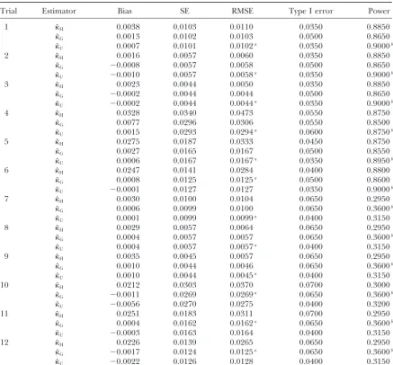
TABLE 1

Comparison of three adjustment factors under␬⫽0.5

Trial Estimator Bias SE RMSE Type I error Power

1 ␬ˆH 0.0038 0.0103 0.0110 0.0350 0.8850

␬ˆG 0.0013 0.0102 0.0103 0.0500 0.8650

␬ˆU 0.0007 0.0101 0.0102a 0.0350 0.9000b

2 ␬ˆH 0.0016 0.0057 0.0060 0.0350 0.8850

␬ˆG ⫺0.0008 0.0057 0.0058 0.0500 0.8650

␬ˆU ⫺0.0010 0.0057 0.0058a 0.0350 0.9000b

3 ␬ˆH 0.0023 0.0044 0.0050 0.0350 0.8850

␬ˆG ⫺0.0002 0.0044 0.0044 0.0500 0.8650

␬ˆU ⫺0.0002 0.0044 0.0044a 0.0350 0.9000b

4 ␬ˆH 0.0328 0.0340 0.0473 0.0550 0.8750

␬ˆG 0.0077 0.0296 0.0306 0.0550 0.8500

␬ˆU 0.0015 0.0293 0.0294a 0.0600 0.8750b

5 ␬ˆH 0.0275 0.0187 0.0333 0.0450 0.8750

␬ˆG 0.0027 0.0165 0.0167 0.0500 0.8550

␬ˆU 0.0006 0.0167 0.0167a 0.0350 0.8950b

6 ␬ˆH 0.0247 0.0141 0.0284 0.0400 0.8800

␬ˆG 0.0008 0.0125 0.0125a 0.0500 0.8600

␬ˆU ⫺0.0001 0.0127 0.0127 0.0350 0.9000b

7 ␬ˆH 0.0030 0.0100 0.0104 0.0650 0.2950

␬ˆG 0.0006 0.0099 0.0100 0.0650 0.3600b

␬ˆU 0.0001 0.0099 0.0099a 0.0400 0.3150

8 ␬ˆH 0.0029 0.0057 0.0064 0.0650 0.2950

␬ˆG 0.0004 0.0057 0.0057 0.0650 0.3600b

␬ˆU 0.0004 0.0057 0.0057a 0.0400 0.3150

9 ␬ˆH 0.0035 0.0045 0.0057 0.0650 0.2950

␬ˆG 0.0010 0.0044 0.0046 0.0650 0.3600b

␬ˆU 0.0010 0.0044 0.0045a 0.0400 0.3150

10 ␬ˆH 0.0212 0.0303 0.0370 0.0700 0.3000

␬ˆG ⫺0.0011 0.0269 0.0269a 0.0650 0.3600b

␬ˆU ⫺0.0056 0.0270 0.0275 0.0400 0.3200

11 ␬ˆH 0.0251 0.0183 0.0311 0.0700 0.2950

␬ˆG 0.0004 0.0162 0.0162a 0.0650 0.3600b

␬ˆU ⫺0.0003 0.0163 0.0164 0.0400 0.3150

12 ␬ˆH 0.0226 0.0139 0.0265 0.0650 0.2950

␬ˆG ⫺0.0017 0.0124 0.0125a 0.0650 0.3600b

␬ˆU ⫺0.0022 0.0126 0.0128 0.0400 0.3150

a_{Denotes the estimator with minimum RMSE among three estimators.} b_{Denotes the estimator with maximum power among three estimators.}

on Equation 7, are shown in Table 4 in columns 4 (Hoo- experiments. Our proposed adjustments reduced the error further than did Hoogendoorn’s method. More-gendoorn’s method), 5 (geometric-mean method), and

6 (bias-reduction method). over, our proposed methods yielded a smaller variation

in the CPA compared with Hoogendoorn’s method, To summarize the findings in this analysis of

labora-tory data, we found that it is essential to adjust for prefer- and in turn our methods gave a smaller variation in allele frequency estimation. Overall, our results demon-ential amplification. This adjustment reduced the

esti-mation bias of the allele frequencies except for the strate that the proposed adjustments provide a more accurate and reliable estimation of allele frequency for second SNP in this data set. In this case, the serious

underestimate of allele frequency might have arisen from this data set. uncontrollable experimental variations, such as

overesti-mation of the extended primer or an effect of DNA

DISCUSSION quality on SNP variance (Werneret al. 2002). For this

specific SNP, the adjustment procedure yielded only Preferential amplification of nucleotides occurs fre-quently in DNA-pooling studies. Therefore, it is critical limited improvement.

In most cases in our study, Hoogendoorn’s method to adjust this interference presented in two nucleotides in the same SNP so as to avoid a severe bias in the allele reduced the discrepancy between the allele frequencies

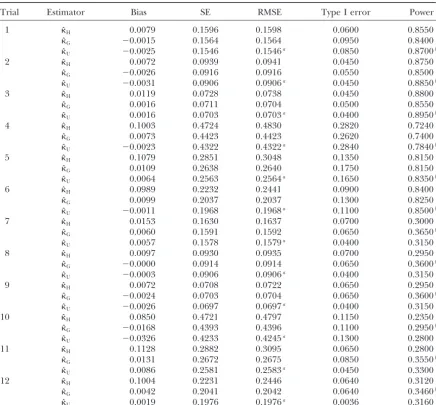
TABLE 2

Comparison of three adjustment factors under␬⫽1

Trial Estimator Bias SE RMSE Type I error Power

1 ␬ˆH 0.0057 0.0343 0.0348 0.0440 0.8680

␬ˆG 0.0013 0.0339 0.0339 0.0460 0.8420

␬ˆU 0.0004 0.0338 0.0338a 0.0400 0.8960b

2 ␬ˆH 0.0023 0.0203 0.0204 0.0350 0.8850

␬ˆG ⫺0.0025 0.0201 0.0202 0.0500 0.8650

␬ˆU ⫺0.0027 0.0199 0.0201a 0.0350 0.9000b

3 ␬ˆH 0.0038 0.0161 0.0165 0.0350 0.8850

␬ˆG ⫺0.0011 0.0159 0.0159 0.0500 0.8650

␬ˆU ⫺0.0013 0.0158 0.0159a 0.0350 0.9000b

4 ␬ˆH 0.0570 0.0910 0.1074 0.0750 0.8600

␬ˆG 0.0079 0.0789 0.0793 0.1000 0.8350

␬ˆU 0.0030 0.0758 0.0758a 0.0850 0.8700b

5 ␬ˆH 0.0421 0.0711 0.0826 0.0550 0.8650

␬ˆG ⫺0.0042 0.0619 0.0620 0.0700 0.8500

␬ˆU ⫺0.0044 0.0599 0.0601a 0.0550 0.8800b

6 ␬ˆH 0.0522 0.0566 0.0770 0.0450 0.8750

␬ˆG 0.0031 0.0492 0.0493 0.0600 0.8500

␬ˆU 0.0021 0.0477 0.0478a 0.0500 0.8900b

7 ␬ˆH 0.0067 0.0337 0.0344 0.0650 0.2950

␬ˆG 0.0024 0.0332 0.0333 0.0650 0.3600b

␬ˆU 0.0015 0.0331 0.0332a 0.0400 0.3150

8 ␬ˆH 0.0048 0.0203 0.0208 0.0650 0.2950

␬ˆG 0.0001 0.0202 0.0202 0.0650 0.3600b

␬ˆU ⫺0.0001 0.0201 0.0201a 0.0400 0.3150

9 ␬ˆH 0.0055 0.0161 0.0170 0.0650 0.2950

␬ˆG 0.0005 0.0159 0.0159 0.0650 0.3600b

␬ˆU 0.0003 0.0158 0.0158a 0.0400 0.3150

10 ␬ˆH 0.0569 0.1264 0.1386 0.0800 0.2750

␬ˆG 0.0110 0.1100 0.1105 0.0790 0.2770

␬ˆU 0.0029 0.1047 0.1048a 0.0680 0.2970b

11 ␬ˆH 0.0555 0.0737 0.0922 0.0700 0.3000

␬ˆG 0.0066 0.0643 0.0646 0.0650 0.3650b

␬ˆU 0.0037 0.0618 0.0619a 0.0400 0.3200

12 ␬ˆH 0.0499 0.0575 0.0761 0.0700 0.2950

␬ˆG ⫺0.0003 0.0499 0.0499 0.0650 0.3600b

␬ˆU ⫺0.0010 0.0483 0.0483a 0.0400 0.3200

a_{Denotes the estimator with minimum RMSE among three estimators.} b_{Denotes the estimator with maximum power among three estimators.}

the power of the association test. In this work, we pro- placed in the denominator when calculating the adjust-ment factor (see Equations 3 and 4).

pose two adjustment methods that improve on the

Hoo-gendoorn’s adjustment (Hoogendoorn et al. 2000). In addition to our two new proposed adjustment fac-tors, we also investigated several other methods, includ-The performance was evaluated by simulation studies.

The new methods yield not only lower bias, standard ing the median-based measure, harmonic-mean-based measure, and some modified ratio estimators (Beale error, and RMSE in allele frequency estimation, but also

better statistical power for genetic association mapping 1962;Tin1965). Although some of these methods yielded a better estimate of CPA than Hoogendoorn’s method under the given test size.

In our method, type I error is usually controlled well did during the simulation study (Yanget al. 2003), they are not superior to our proposed adjustment factors in except when the CV of the peak intensity is high and

␬ ⬎1. Also, the performance of␬ˆ is apparently not sym- this article.

We investigated the role of sample size during the metric when␬ ⫽1. In general, a smaller CPA yields a

correspondingly smaller RMSE. Regarding the instances pilot stage of the DNA-pooling study. The use of a large number of heterozygous individuals reduces the RMSE of␬ ⫽2 and␬ ⫽0.5, the latter gives better performance

TABLE 3

Comparison of three adjustment factors under␬⫽2

Trial Estimator Bias SE RMSE Type I error Power

1 ␬ˆH 0.0079 0.1596 0.1598 0.0600 0.8550

␬ˆG ⫺0.0015 0.1564 0.1564 0.0950 0.8400

␬ˆU ⫺0.0025 0.1546 0.1546a 0.0850 0.8700b

2 ␬ˆH 0.0072 0.0939 0.0941 0.0450 0.8750

␬ˆG ⫺0.0026 0.0916 0.0916 0.0550 0.8500

␬ˆU ⫺0.0031 0.0906 0.0906a 0.0450 0.8850b

3 ␬ˆH 0.0119 0.0728 0.0738 0.0450 0.8800

␬ˆG 0.0016 0.0711 0.0704 0.0500 0.8550

␬ˆU 0.0016 0.0703 0.0703a 0.0400 0.8950b

4 ␬ˆH 0.1003 0.4724 0.4830 0.2820 0.7240

␬ˆG 0.0073 0.4423 0.4423 0.2620 0.7400

␬ˆU ⫺0.0023 0.4322 0.4322a 0.2840 0.7840b

5 ␬ˆH 0.1079 0.2851 0.3048 0.1350 0.8150

␬ˆG 0.0109 0.2638 0.2640 0.1750 0.8150

␬ˆU 0.0064 0.2563 0.2564a 0.1650 0.8350b

6 ␬ˆH 0.0989 0.2232 0.2441 0.0900 0.8400

␬ˆG 0.0099 0.2037 0.2037 0.1300 0.8250

␬ˆU ⫺0.0011 0.1968 0.1968a 0.1100 0.8500b

7 ␬ˆH 0.0153 0.1630 0.1637 0.0700 0.3000

␬ˆG 0.0060 0.1591 0.1592 0.0650 0.3650b

␬ˆU 0.0057 0.1578 0.1579a 0.0400 0.3150

8 ␬ˆH 0.0097 0.0930 0.0935 0.0700 0.2950

␬ˆG ⫺0.0000 0.0914 0.0914 0.0650 0.3600b

␬ˆU ⫺0.0003 0.0906 0.0906a 0.0400 0.3150

9 ␬ˆH 0.0072 0.0708 0.0722 0.0650 0.2950

␬ˆG ⫺0.0024 0.0703 0.0704 0.0650 0.3600b

␬ˆU ⫺0.0026 0.0697 0.0697a 0.0400 0.3150

10 ␬ˆH 0.0850 0.4721 0.4797 0.1150 0.2350

␬ˆG ⫺0.0168 0.4393 0.4396 0.1100 0.2950b

␬ˆU ⫺0.0326 0.4233 0.4245a 0.1300 0.2800

11 ␬ˆH 0.1128 0.2882 0.3095 0.0650 0.2800

␬ˆG 0.0131 0.2672 0.2675 0.0850 0.3550b

␬ˆU 0.0086 0.2581 0.2583a 0.0450 0.3300

12 ␬ˆH 0.1004 0.2231 0.2446 0.0640 0.3120

␬ˆG 0.0042 0.2041 0.2042 0.0640 0.3460b

␬ˆU 0.0019 0.1976 0.1976a 0.0036 0.3160

a_{Denotes the estimator with minimum RMSE among three estimators.} b_{Denotes the estimator with maximum power among three estimators.}

ment factor. To explore the sample size requirement, screening for important genetic variants at a reasonable cost. However, the unavoidable drawback is that geno-we considered both fixed-effect and random-effect

mod-els for different scenarios. In general, random-effect typic information and individual features are lost once genomic DNA is mixed. Although some advanced stud-models yield a larger sample size than fixed-effect

mod-els when the same set of parameters is used. For exam- ies have attempted to reconstruct the lost information (Itoet al. 2003), a bottleneck still exists due to the mass ple, given that the genotype frequency in the population

is 0.45 and 8 heterozygous individuals are required, 21 of genotype and haplotype combinations in the pool. Stringent limitations must be satisfied for small pools individuals need to be genotyped under the fixed-effect

model [i.e., CV(pAa) ⫽ 0]; 24 and 34 individuals need to reduce the number of combinatorial calculations. To

date, DNA-pooling experiments have been used primar-to be genotyped under CV(pAa)⫽0.25 and 0.5,

respec-tively, in the random-effect model. This is so because the ily as a screening technique rather than as a legitimate replacement for individual genotyping studies.

random-effect models take into consideration variations

among individuals, resulting in an increase in total varia- Use of DNA pooling is a potentially cost-effective alter-native to individual genotyping. Association testing in tion that requires a larger sample size to compensate.

Ignoring the heterogeneity may lead to a serious under- DNA pools is an efficient method for screening impor-tant genetic markers and has been applied successfully estimation of sample sizes.

TABLE 4

Comparisons of estimated allele frequencies from individual genotyping, the pooling experiment without adjustment, and the pooling experiments using different adjustments

Individual Without Adjustment Adjustment Adjustment

SNP genotyping adjustment ␬ˆH ␬ˆG ␬ˆU

1 0.067 0.055 0.073 0.072 0.070

2 0.217 0.034 0.040 0.050 0.051

3 0.233 0.163 0.227 0.235 0.236

4 0.250 0.357 0.327 0.323 0.321

5 0.383 0.183 0.283 0.281 0.285

6 0.433 0.194 0.355 0.353 0.359

Sham, P., J. S. Bader, I. Craig, M. O’DonovanandM. Owen, 2002

conclusions (Carmiet al. 1995;Bansalet al. 2002). Our

DNA pooling: a tool for large-scale association studies. Nat. Rev.

new approaches provide valid adjustments and further _{Genet.3:862–871.}

Tin, M., 1965 Comparison of some ratio estimators. J. Am. Stat.

improve the conventional method, thereby the reliable

Assoc.60:294–307.

allele frequency estimation and powerful association

Visscher, P. M., andS. Le Hellard, 2003 Simple method to analyze

tests. These advantages enhance greatly the applicability _{SNP-based association studies using DNA pools. Genet.}

Epide-miol.24:291–296.

of the DNA-pooling experiment.

Werner, M., M. Sych, N. Herbon, T. Illig, I. R. Koniget al., 2002

We thank Jer-Yuan Wu and the National Genotyping Center and _{Large-scale determination of SNP allele frequencies in DNA pools}

National Clinical Core at Academia Sinica for genotyping support. _{using MALDI-TOF mass spectrometry. Hum. Mutat.20:57–64.}

We appreciate the two anonymous reviewers for providing insightful Yang, H.-C., C.-L. ChenandC. S. J. Fann, 2003 Estimation of allele

frequencies with preferential amplification in a DNA-pooling suggestions and comments, which have greatly enhanced the

presenta-study. Am. J. Hum. Genet.73:2625.

tion of this article. This research was supported by a National Science Council grant (NSC 92-3112-B-001-014) and an Academia Sinica grant

Communicating editor: R. W.Doerge

(93IBMS2PP-C) of Taiwan.

APPENDIX A: PROPERTIES OF THE PROPOSED

LITERATURE CITED _{ADJUSTMENT FACTOR}

Bansal, A., D. Van Den Boom, S. Kammerer, C. Honisch, G. Adam

Suppose that the population size of heterozygous indi-et al., 2002 Association testing by DNA pooling: an effective

initial screen. Proc. Natl. Acad. Sci. USA99:16871–16874. viduals is Nheter and nheter samples are randomly drawn

Barratt, B. J., F. Payne, H. E. Rance, S. Nutland, J. A. Toddet al., _{from the population. Letr(j)⫽h}I

A(j)/hIa(j). Hence,

2002 Identification of the sources of error in allele frequency

the bias of Hoogendoorn’s measure can be calculated

estimations from pooled DNA indicates an optimal experimental

design. Ann. Hum. Genet.66:393–405. using the following:

Beale, E. M. L., 1962 Some uses of computers in operational

re-search. Indust. Organ.31:51–52.

␭ ⫽E(␬ˆH)⫺ ␬ ⫽E

冢

n⫺heter1

兺

nheter

j⫽1

[hI

A(j)/hAI(j)]

冣

⫺ ␬

Carmi, R., T. Rokhlina, A. E. Kwitek-Black, K. Elbedour, D. Nishi-muraet al., 1995 Use of a DNA pooling strategy to identify a human obesity syndrome locus on chromosome 15. Mol. Genet.

4:9–13. _⫽

N⫺1 heter

兺

N_heter

j⫽1

[hI

A(j)/hIa(j)]⫺HA/Ha

Downes, K., B. J. Barratt, P. Akan, S. J. Bumpstead, S. D. Taylor et al., 2004 SNP allele frequency estimation in DNA pools and

variance components analysis. Biotechniques36:840–845.

⫽(NheterHa)⫺1

兺

N_heter

j⫽1

{r(j)Ha}⫺

兺

N_heter

j⫽1

[r(j)hI

a(j)]/Ha

Efron, B., andR. J. Tibshirani, 1993 An Introduction to the Bootstrap. Chapman & Hall, New York.

Hartley, H. O., and A.Ross, 1954 Unbiased ratio estimates. Nature

174:270–271. _⫽(N

heterHa)⫺1⫻

兺

Nheter

j⫽1

{r(j)Ha}⫺ (NheterHa)⫺1

Hoogendoorn, B., N. Norton, G. Jirov, N. Williams, M. L. Ham-shereet al., 2000 Cheap, accurate and rapid allele frequency estimation of single nucleotide polymorphisms by primer

exten-⫻ Nheter

兺

N_heter

j⫽1

[r(j)hI a(j)]

sion and DHPLC in DNA pools. Hum. Genet.107:488–493.

Ito, T., S. Chiku, E. Inoue, M. Tomita, T. Morisakiet al., 2003 Estimation of haplotype frequencies, linkage-disequilibrium

mea-sures, and combination of haplotype copies in each pool by use _⫽(N

heter␮a)⫺1

兺

N_heter

j⫽1

r(j)[␮a⫺hIa(j)].

of pooled DNA data. Am. J. Hum. Genet.72:384–398.

Le Hellard, S., S. J. Ballereau, P. M. Visscher, H. S. Torrance,

J. Pinsonet al., 2002 SNP genotyping on pooled DNAs: compari- _{We used the estimated bias} son of genotyping technologies and a semi-automated method

for data storage and analysis. Nucleic Acids Res.30:e74. _{␭ˆ ⫽(h}I

a)⫺1⫻(nheter⫺ 1)⫺1 ⫻nheter⫻ (␬ˆhIa⫺ hIA)

Mohlke, K. L., M. R. Erdos, L. J. Scott, T. E. Fingerlin, A. U. Jacksonet al., 2002 High-throughput screening for evidence

to correct the bias in Hoogendoorn’s method. This

esti-of association by using mass spectrometry genotyping on DNA

to the consideration of finite population in Hartley Hence, the marginal distribution ofntotalcan be derived

as follows: andRoss(1954).

f(ntotal)⫽

冮

1

0

冢

ntotal⫺1

nheter⫺1

冣

(2pApa)nheter(1⫺2pApa)nhomo APPENDIX B: SAMPLE SIZE CALCULATION

IN A PILOT STUDY

⫻(pA)␪⫺1(1⫺pA)␶⫺1

B(␪,␶) dpA Suppose that the estimated allele frequencypˆis a

dif-ferentiable function of␬ˆ andhP

A/hPaat a point (␬,HA/Ha).

By a first-order Taylor expansion of two variables␬ˆ and

⫽

冢

ntotal⫺1

nheter⫺1

冣

2nheter

B(␪,␶)

冮

1

0

(pA)nheter⫹␪⫺1(1⫺pA)nheter⫹␶⫺1

hP

A/hPa at (␬,HA/Ha), we know that

pˆ⫽ p⫺{p2_/(H

A/Ha)}(␬ˆ ⫺ ␬)

⫻

_兺

nhomo

y⫽0

冢

nhomo

y

冣

(⫺1)

y_(2p Apa)ydpA

⫹p2_{␬_/(H

A/Ha)2}(hPA/haP⫺HA/Ha)⫹ R1,

where ␩ ⫽(␬ˆ ⫺ ␬,hP

A/hPa ⫺HA/Ha) and satisfies R1/ _⫽

冢

ntotal⫺1

nheter⫺1

冣

2nheter

B(␪,␶)

兺

nhomo

y⫽0

冢

nhomo

y

冣

(⫺1)

y₂y

||␩||→0 as ||␩||→0. The approximate mean and vari-ance can be calculated as

⫻B(nheter⫹y⫹ ␪,nheter⫹y⫹ ␶).

E(pˆ)⬇p

Under the RGF model, we assume genotype frequency

and pAafollows from a beta distribution beta(␪,␶). The

mar-ginal distribution ofntotalis

Var(pˆ)⬇p2₍₁ ⫺_p)2_CV2

␬ˆ ⫹

␬2_p4

(HA/Ha)2

CV2hP

A/hPa,

f(ntotal)⫽

冮

1

0

冢

ntotal⫺1

nheter⫺1

冣

(pAa)nheter(1⫺pAa)nhomo

where CV2

␬ˆ ⫽V(␬ˆ)/␬2and CV 2

hAP/hPa⫽V(h

P

A/hPa)/(HA/Ha)2.

The pure variation due to the adjustment of preferential _⫻(pAa)␪⫺1(1⫺pAa)␶⫺1

B(␪,␶) dpAa amplification can be obtained by settinghP

A/hPa ⫽HA/Ha,

resulting in the following variance:

⫽

冢

ntotal⫺1

nheter⫺1

冣

1

B(␪,␶)

冮

1

0

(pAa)nheter⫹␪⫺1(1⫺p_Aa)nhomo⫹␶⫺1dp_Aa Var(ε␬ˆ)⬇p2(1 ⫺p)2CV2␬ˆ. (B1)

If␬ˆ ⫽ ␬, then we obtain the pure variance due to the _⫽

冢

ntotal⫺1

nheter⫺1

冣

B(␪ ⫹nheter,␶ ⫹nhomo)

B(␪,␶) . measurement of the ratio of the peak intensities,

Second, under large-scale genotyping experiments,nheter

Var(pˆ|␬ˆ ⫽ ␬)⬇ ␬

2_p4

(HA/Ha)2

CV2hPA/hPa. _{is a random variable that follows a binomial distribution}

with successful probabilitypH. Under the beta-binomial

To calculate the required samples size, the variance

random allele frequency model, the marginal distribu-in Equation B1 must be rewritten as a function ofnheter. _{tion ofn}

heteris

If the adjustment ofHoogendoornet al. (2000) is ap-plied, then the variance in Equation B1 can be

repre-f(nheter)⫽

冮

1

0

冢

ntotal

nheter

冣

(2pApa)nheter(1⫺2pApa)nhomo

sented as

Var(ε_␬ˆ)⬇p2(1⫺ p)2(CV2r/nheter),

⫻(pA)␪⫺1(1⫺pA)␶⫺1

B(␪,␶) dpA where CV2

r ⫽V(rj)/␬2 and rj⫽hIA(j)/haI(j), j⫽ 1, . . . ,

nheter. Under risk␣ and the specified absolute error␰,

the required number of heterozygous individuals is ⫽

冢

ntotal

nheter

冣

2n_heter

B(␪,␶)

兺

n_homo

y⫽0

冢

nhomo

y

冣

(⫺1)

y₂y

nheter⫽{[t1⫺␣/2p(1 ⫺p)CVr]␰⫺1}2,

⫻B(nheter⫹y⫹ ␪,nheter⫹y⫹ ␶).

whereP{|p(␬ˆ)⫺ p|⬍ ␰}ⱖ 1⫺ ␣.

Under the beta-binomial random genotype frequency model, the marginal distribution ofnheteris

APPENDIX C: THE MARGINAL DISTRIBUTIONS OF SAMPLE SIZES UNDER DIFFERENT

f(nheter)⫽

冮

1

0

冢

ntotal

nheter

冣

(pAa)nheter(1⫺pAa)nhomo GENOTYPING EXPERIMENTS

First, under sequential genotyping experiments,ntotal

⫻(pAa)␪⫺1(1 ⫺pAa)␶⫺1

B(␪,␶) dpAa is a random variable that follows a negative binomial

dis-tribution with successful probability pH(probability of

heterozygote). Under the RAF model, we assume allele

⫽

冢

ntotal

nheter

冣

B(␪ ⫹nheter,␶ ⫹nhomo)