DOI: 10.1534/genetics.107.071142
Bayesian Mapping of Genomewide Interacting Quantitative Trait Loci
for Ordinal Traits
Nengjun Yi,*
,1Samprit Banerjee,* Daniel Pomp
†and Brian S. Yandell
‡*Section on Statistical Genetics, Department of Biostatistics, University of Alabama, Birmingham, Alabama 35294,†Department of Nutrition and Department of Cell and Molecular Physiology, University of North Carolina, Chapel Hill, North Carolina 27599 and
‡Department of Statistics and Department of Horticulture, University of Wisconsin, Madison, Wisconsin 53706
Manuscript received January 18, 2007 Accepted for publication May 11, 2007
ABSTRACT
Development of statistical methods and software for mapping interacting QTL has been the focus of much recent research. We previously developed a Bayesian model selection framework, based on the composite model space approach, for mapping multiple epistatic QTL affecting continuous traits. In this study we extend the composite model space approach to complex ordinal traits in experimental crosses. We jointly model main and epistatic effects of QTL and environmental factors on the basis of the ordinal probit model (also called threshold model) that assumes a latent continuous trait underlies the generation of the ordinal phenotypes through a set of unknown thresholds. A data augmentation approach is developed to jointly generate the latent data and the thresholds. The proposed ordinal probit model, combined with the composite model space framework for continuous traits, offers a convenient way for genomewide interacting QTL analysis of ordinal traits. We illustrate the proposed method by detecting new QTL and epistatic effects for an ordinal trait, dead fetuses, in a F2intercross of mice. Utility
and flexibility of the method are also demonstrated using a simulated data set. Our method has been implemented in the freely available package R/qtlbim, which greatly facilitates the general usage of the Bayesian methodology for genomewide interacting QTL analysis for continuous, binary, and ordinal traits in experimental crosses.
M
OST complex traits are influenced by interacting networks of multiple genetic (QTL) and envi-ronmental factors. Recently several statistical methods and software have been developed to map multiple interacting QTL for continuous traits (Kaoet al.1999;Carlborget al.2000; Reifsnyderet al.2000; Bogdan et al.2004; Yiet al.2005; Baierlet al.2006). However,
many complex traits in humans and other organisms are measured in an ordinal manner. For example, many diseases are scored in several ordered categories on the basis of the magnitude of the disease symptom. Although the phenotypes of these characters are discrete, their inheritance is determined by many factors, including multiple genes and environmental components (Lynch
and Walsh1998). Theoretically, the statistical methods
for continuous traits are not optimal for ordinal traits because the normality assumption is violated ( Johnson
and Albert1999; Gelmanet al.2003). Therefore,
map-ping QTL for ordinal traits requires new methods. The probit model is commonly used to analyze dis-crete binary and ordinal data (Albertand Chib1993;
Johnsonand Albert1999). An important way for the
statistical inference and interpretation of the probit model is to postulate the existence of a latent (unob-served) continuous variable associated with each re-sponse through a series of unknown thresholds (Albert
and Chib1993; Johnsonand Albert1999). In
quan-titative genetics, the latent presentation of the probit model is called the threshold model, which has been widely used to analyze the genetic architecture of binary and ordinal traits (Wright 1934; Lynchand Walsh
1998). Under the threshold model, one can treat the latent variable as an unobservable quantitative trait, and genes controlling ordinal traits can be treated as quan-titative trait loci and handled using a QTL mapping approach.
A number of statistical methods have been developed to identify QTL for binary or ordinal traits in experi-mental crosses based on the threshold model of single QTL (Hackett and Weller 1995; Xu and Atchley
1996; Raoand Xu1998; Xuet al.2003, 2005). Recently,
several methods have been proposed to simultaneously identify multiple QTL for ordinal traits (Coffmanet al.
2005; Liet al.2006). The method of Liet al.(2006) is
based on multiple-interval mapping (MIM) of Kaoet al.
(1999) that fits a multiple-QTL model including epista-sis and simultaneously searches for the number, posi-tions, and interaction of QTL using a non-Bayesian model selection procedure and criterion.
1Corresponding author:Section on Statistical Genetics, Department of
Biostatistics, University of Alabama, Birmingham, AL 35294-0022. E-mail: [email protected]
Several studies have extended Bayesian methods of mapping multiple QTL for continuous traits to binary traits on the basis of the threshold model of multiple QTL. Yi and Xu (2000) first developed a Bayesian
method via a reversible-jump Markov chain Monte Carlo (MCMC) algorithm to map multiple QTL for binary traits. The method of Yiand Xu(2000) is based on the
idea of data augmentation, allowing an easy way to extend the existing Bayesian mapping methods to bi-nary traits. Recently, Yi et al. (2004) extended the
Bayesian mapping method via a reversible-jump MCMC algorithm to map multiple nonepistatic QTL for ordinal traits. However, Bayesian methods of mapping interact-ing QTL for ordinal traits are lackinteract-ing. Even for con-tinuous traits, identification of genomewide interacting QTL has been a formidable challenge, mainly due to numerous possible variables associated with hundreds or thousands of genomic loci that lead to a huge number of possible models.
In this study we propose a Bayesian model selection approach of genomewide interacting QTL for ordinal traits in experimental crosses. We first develop a Bayesian ordinal probit model (threshold model) for multiple interacting QTL, on the basis of the composite model space framework proposed by Yiet al.(2005). Our
ordinal probit model simultaneously considers main and epistatic effects of QTL and environmental factors. We then use the composite model space framework to develop an efficient MCMC algorithm for identifying interacting QTL for ordinal traits. The composite mo-del space approach was proposed by Yi(2004) for
map-ping multiple nonepistatic QTL and extended by Yiet al.
(2005) to epistatic QTL mapping for continuous traits. The key advantage of the composite model space approach is that it provides a convenient way to reaso-nably reduce the model space and to construct efficient algorithms for exploring the complicated posterior dis-tribution. Utility and flexibility of the method are de-monstrated using real and simulated data sets.
BAYESIAN MODELING OF ORDINAL TRAITS
Ordinal data modeling via latent variables: Assume that we observe an ordinal phenotype in a mapping population. The property of ordinal data is that there exists a clear ordering of the response categories, but no underlying interval scale between them ( Johnsonand
Albert1999). For example, it is usual to record disease
severity using an ordinal character system that assesses the extent of the disease. Although one may record the ordinal categories as (arbitrarily) numeric values, it does not always make sense to do so. Even if numeric scores are used, it is not appropriate to apply the sta-tistical methods for continuous data to ordinal data be-cause the normality assumption is violated.
The ordinal probit model is commonly used to analyze ordinal data (Albertand Chib1993; Johnson
and Albert 1999). Let wi be the ordinal phenotype
andxithe relevant explanatory variables for theith
in-dividual in an experimental cross of sample sizen. For notational convenience, we code the ordinal data as the integers 1, 2, , J, with J the number of categories. Under the ordinal probit model, the data distribution takes the form
pðwi¼jjxi;b;s2;tÞ ¼F
tjxib
s
F tj1xib s
;
ð1Þ
where FðÞ is the standardized normal distribution function,brepresents the overall mean and regression coefficients, s2 is the residual variance, and ‘¼
t0#t1# #tJ1#tJ ¼ 1‘are unknown thresholds.
An important idea for interpreting and computing the ordinal probit model involves reexpressing model (1) in terms of unobserved (latent) continuous data (Albert and Chib 1993). Let yi represent the latent
variable that underlies the generation of the ordinal response for the ith individual. The ordinal probit model is equivalent to the following model on latent datayi,
yi¼xib1ei
wi ¼jÛtj1#yi,tj ð2Þ
withei,i¼1, ,n, independently normal with mean
zero and variances2.
The advantage of the latent parameterization for the probit model is that it offers a convenient framework for MCMC simulation. Conditional on the parameters (b, s2,t) and the observed data, the distribution ofy
ifollows
a truncated normal distribution that can be easily sam-pled. Conditional on the latent yi’s, the model is a
normal linear regression and thus the posterior distri-bution of the model parameters (b, s2) can be
com-puted using standard results for normal linear models (Albertand Chib1993; Johnsonand Albert1999; Yi et al.2004).
Model (1), or (2), is overparameterized. There are usually two ways to impose restrictions on the parame-ters that can ensure identifiability. The first is to sett1¼0
ands2¼1, so that there areJ2 unknown thresholds
(Albert and Chib 1993). An alternative approach,
which we use here, is to sett1¼0 andtJ1¼1, leaving
s2as a parameter (Chenand Dey2000; Yiet al.2004).
This latter approach has several attractive features, notably that threshold values are between 0 and 1.
Ordinal probit model of multiple interacting QTL:
additional loci, or pseudomarkers (Senand Churchill
2001), between flanking markers. We calculate the probabilities of genotypes at these preset loci given the observed marker data as priors of QTL genotypes in our Bayesian framework.
We place an upper bound on the number of QTL included in the model. This upper bound is larger than the number of detectable QTL with high probability for a given data set. Even with a moderate number of the upper bound, there are many possible genetic effects when considering interactions, but most are negligible and can be excluded. We use an unobserved vector of binary variablesgto indicate which main and epistatic effects across the possible loci are included in (gj¼1) or
excluded from (gj¼0) the model. The indicator vector
g determines the number of included QTL and the activity of the associated genetic effects. We denote the positions of the included QTL byl. The vector (g,l) thus determines the genetic architecture, the number and position of QTL, and their gene action. The goal of our Bayesian approach is to infer the posterior distri-bution of (g, l) and estimate the associated genetic effects.
We simultaneously model main and epistatic effects of QTL and environmental variables (covariates). We include those (continuous or discrete) covariates that may be important in understanding the effect of genotype on phenotype in the model (e.g., sex, family indicators, and some other traits correlated to the phenotype under study). Including relevant covariates can account for systematic or confounding effects that cannot be controlled experimentally. We use Cockerham’s genetic model to construct main effects and epistasis, although other models are possible (Kao and Zeng
2002; Zenget al.2005), and apply conventional
meth-ods used in hierarchical linear models to construct environmental effects (e.g., Lynch and Walsh 1998;
Gelmanet al.2003).
Suppose all genotypes are known across the genome. We can imagine a large design matrixD including all possible effects given the upper bound on the number of QTL. However, given any particularg, we need focus only on a reduced matrix DG ¼ X, identified by the genetic architecture (technically,Gis a matrix contain-ing only those columns of the identity matrix for which g ¼ 1). We partition the design matrix into environ-mental, main, and epistatic effects,X¼ ½XE: XG: XGG,
and express the phenotypeyas
y¼m1XEbE1XGbG1XGGbGG1e¼m1Xb1e
wi ¼jÛtj1#yi,tj; ð3Þ
where wi 2 f1; ;Jg, i ¼ 1, , n, is the observed
ordinal phenotype in a mapping population of n
individuals,y ¼(y1, ,yn) is the unobserved
contin-uous data, ‘¼t0#t1 ¼0#t2# #tJ2#tJ1¼
1#tJ ¼ 1‘are the thresholds, m¼(m, ,m)Tis the
vector of overall mean m, bErepresents the vector of
environmental effects, bG and bGG represent the
vectors of selected main effects and epistatic effects, respectively, andeis the vector of independent normal errors with mean zero and variance s2. To simplify
notation, we organize all effects into band all design matrices intoX.
Prior distributions:We organize the unknowns in the above model into two sets, the parameters that also appear in the corresponding model for continuous traits and the additional parameters. The first set of unknowns includes the indicatorsg, positions of QTLl, QTL genotypes g, regression coefficients b, overall meanm, and residual variances2(Yiet al. 2005). The
QTL genotypes, g, determine the design matrices XG
andXGG. The additional unknowns include the latent
continuous datay¼(y1, ,yn) and the thresholdst¼
(t2, ,tJ2).
For the parameters (g,l,g,m,s2), we use the priors
proposed in Yiet al.(2005). Priors on environmental
effects in bE are assigned uniform distributions or
normal distributions with mean 0 and unknown varian-ces, labeled fixed or random effects from the non-Bayesian tradition, respectively (Gelman et al. 2003).
For the unknown variances, we use conjugate priors, scaled inverse-x2. We take uniform prior on the
un-known thresholdst¼ ðt2; ;tJ1Þ;i.e.,pðtÞ}1, with the
constraint 0,t2, ,tJ2,1.
Hierarchical priors on genetic effects: We here suggest new priors on genetic effects (bG, bGG) that
can restrict their values in a reasonable region and thus induce increased posterior probability on more prom-ising models. We want effect priors that are invariant to the scales of the phenotype and the contrasts in model (3). This can be accomplished by hierarchical models in which the priors have empirical hyperpriors depending on the proportion of liability variance explained by the effect. We partition the genetic effects into batches, corresponding to different types of effects,e.g., additive, dominance, additive–additive interactions, etc. Effects in the same batch k, bkj, follow the same prior, bkjNð0;s2
kÞ. The prior variances
2
kis random with an
inverse-x2 hyperprior, s2
kInv-x
2ðn
k;sk2Þ. The degrees
of freedomnkand scale hyperparameterssk2are chosen
to control the prior expected mean and the prior confidence region of the proportion of the liability variance explained bybkj. The proportion of the liability
variance explained bybkjis thenhkj ¼Vkjb2kj=Vy, withVkj
the sample variance for the column of X associated with effect bkj and Vy the total liability variance. The
prior expectations are EðhkjÞ ¼Vkjsk2=Vy and Eðs2kÞ ¼
nks2k=ðnk2Þ. Setting sk2 ¼ (nk 2)/nk E(hkj)Vy/Vkj
yields E(hkj) as the prior expectation of variance
explained by bkj. E(hkj) can be set small (say 0.05–0.2)
to reflect any prior knowledge about genetic architec-ture. The prior degrees of freedomnkcontrol the skew of the prior for s2
(herenk¼6) to tightly center the prior aroundsk2(see
Chipman2004).
MCMC SAMPLING
Given the prior distributions of all unknowns and the observed data, the joint posterior density can be ex-pressed as
pðy;t;u;cjwÞ}Y
n
i¼1
pðyiju;wi;tÞ pðtÞ pðu;cÞ ð4Þ
withw¼(w1, ,wn) the observed ordinal data,u¼(g,
l,g,bm,s2), andcrepresents all variance parameters
for b. For notational convenience, we suppress the dependence on marker data and covariates here and in subsequent notation.
From model (3), the conditional distribution of the latent variableyi follows a truncated normal
distribu-tion;i.e.,
pðyiju;wi;tÞ ¼f
yimXib
s
Iðtwi1#yi,twiÞ;
ð5Þ
where f denotes the standard normal density, Xi is
theith row ofX, andIðAÞis an indicator function for eventA.
The latent parameterization for the ordinal probit model of multiple interacting QTL allows a convenient sampling approach for simulating from the joint poste-rior of the unknowns (u, c, y, t). Conditional on the latent data yi’s, model (3) becomes the
multiple-interacting-QTL model for continuous traits ½the first line in model (3)and thus the first set of unknownsu can be updated using the sampling methods for con-tinuous traits described in Yiet al.(2005). All elements
of c can be sampled from independent inverse-x2
distributions (Gelmanet al.2003). Therefore, we need
only an additional step to update the additional unknownsyandt. As described below,yandtcan be jointly sampled from the joint conditional posteriorp(y,
tju,w).
We factor the joint conditional posterior of (y,t) into the product
pðy;tju;wÞ ¼pðtju;wÞY
n
i¼1
pðyiju;wi;tÞ: ð6Þ
This factorization suggests that we can first draw the threshold valuestfromp(tju,w) and then drawyifrom
p(yiju,wi,t),i¼1, ,n. The distributionp(yiju,wi,t) is
the normal distribution Nðm1Xib;s2Þ truncated to
the region½twi1;twiÞ. This truncated normal distribu-tion can be sampled using the inverse transformadistribu-tion method (Yiet al. 2004). The first term in (6) can be
obtained as
pðtju; wÞ}Y
n
i¼1
F twimXib s
F twi1mXib s
; ð7Þ
where FðÞ is the standardized normal distribution function. A Metropolis–Hastings step is used to sample from this conditional posterior distribution. To update
tj,j¼2, ,J2, we first sample a new thresholdtj*
uniformly from the interval½max(tj1,tjd), min(tj11, tj1d), wheredis a predetermined tuning parameter,
andtj1, tj, andtj11are the values. The proposaltj* is
then accepted with probability min{1,r}, where
r ¼pðt *ju;wÞ
pðtju;wÞ; ð8Þ
wheretare the current values of the thresholds andt* represents all elements oftexcepttjis replaced bytj*.
The MCMC algorithm described above is used to simulate a Markov chain from the joint posterior, called the posterior sample, (y, t, u, c)(1), (y, t,u,c)(2), ,
which converges to the joint posteriorp(y,t,u,cjw) (Chipmanet al.2001). The posterior sample can be used
to infer the genetic architecture of the ordinal trait, including the number and locations of QTL and their main and epistatic effects. The idea is that larger effects should tend to appear more often and early in a sample from the Markov chain, making them easier to identify. Our basic principle for posterior inference is to use all the saved iterations of the Markov chain, corresponding to model averaging, which assesses characteristics of the genetic architecture by averaging over possible models weighted by their posterior probabilities. Model averag-ing accounts for model uncertainty and hence provides more robust inference compared to a single ‘‘best’’ model approach (Raftery et al. 1997; Ball 2001;
Sillanpa¨ a¨and Corander2002).
We can use various methods to graphically and nu-merically summarize and interpret the posterior sam-ples. The posterior inclusion probability for each locus is estimated as its frequency in the posterior samples. Each locus may be included in the model through its main effects and/or interactions with other loci (epis-tasis). The larger the effect size is for a locus, the more frequently the locus is sampled. Taking the prior pro-bability into consideration, we use Bayes factors (BF) to show evidence for inclusion against exclusion of a locus. The Bayes factor for a locus is defined as the ratio of the posterior odds to the prior odds for inclusion against exclusion of the locus (Kass and Raftery 1995).
Traditionally, a BF threshold of 3, or 2 loge(BF)¼2.1,
supports a claim of significance (Kass and Raftery
IMPLEMENTATION IN R/QTLBIM
We have implemented the methods proposed herein in the freely available package R/qtlbim (Yandellet al.
2007). R/qtlbim is an extensible, interactive environ-ment for Bayesian analysis of multiple interacting QTL for continuous, binary, and ordinal traits in experimen-tal crosses. It is built on the widely used R/qtl package (Bromanet al.2003) and includes all its advantages for
extensibility. In R/qtlbim, the computationally inten-sive MCMC algorithms are written in C, with data manipulation and graphics in R. The algorithms for ordinal traits use the same C functions for continuous traits to update the first set of unknowns u, with additional functions for jointly updating the latent data
yand the thresholdst.
R/qtlbim provides tools to monitor mixing behavior and convergence of the simulated Markov chain, either by examining trace plots of the sample values of scalar quantities of interest, such as the numbers of QTL and epistatic effects, or by using formal diagnostic methods provided in the package R/coda (Plummeret al. 2004).
The posterior summaries for ordinal traits are the same as those for continuous traits, because all the parame-ters of interest are included in the set of unknownsu. R/ qtlbim provides extensive informative graphical and numerical summaries of the MCMC output to infer and interpret key aspects of the genetic architecture (Yandellet al.2007).
MAPPING INTERACTING QTL FOR FETUSES IN MICE
We illustrate our method by reanalyzing a reproduc-tive trait from a QTL study done by Rochaet. al(2004).
Ten-week-old F2 females, of a cross between a
high-growth M16i line and the low-body-weight L6 line, were exposed to unrelated F1 males (B6C3F1/J) until a
copulatory plug was detected. Both M16i and L6 mice were inbred lines. Pregnant females (n ¼ 439) were subsequently euthanized at day 16 of gestation to obtain dead fetuses (DF) and several other reproductive phenotypes. Body weights at 10 weeks of age (WK10) were also measured. WK10 was significantly correlated with DF. These F2female mice encompass two
consec-utive replicates consisting of 217 and 222 mice, re-spectively, and 65 full-sib families/litters ranging from 1 to 11 mice. A total of 63 fully informative microsatellite markers spanning 19 autosomes were genotyped. The marker linkage map covered 1257.8 cM (Kosambi) with an average spacing of 30 cM. The observed DF took integral values ranging from 0 to 11 (Figure 1). We discarded 5 mice having .6 (7, 8, 10, and 11) dead fetuses that may be outliers.
In spite of their conformity to an ordinal character, this F2data set was previously analyzed in Rochaet al.
(2004), using standard composite-interval mapping (Zeng1994) treating DF as continuous traits. The
pre-vious analysis first performed an ad hoc square-root transformation for the ordinal trait DF and then used residuals as a new phenotype obtained by linearly adjusting the effects of replicates and family. Rocha et al.(2004) reported a single significant (LOD¼4.4) QTL on chromosome 2 (position 41.6 cM) for DF.
DF is the natural phenotype of interest to exhibit the effectiveness of our proposed method in handling ordinal traits. In our Bayesian analysis, our model in-cluded WK10 and replicates as fixed continuous and discrete covariates, respectively, and family indicators as a random categorical covariate. We permitted the inclu-sion of epistatic effects in the model. We used Cocker-ham’s genetic model to construct genetic effects, in which the additive and dominance contrasts are defined as (1, 0, 1) and (0.5, 0.5,0.5) for the three geno-types, LL, ML, and MM, where L and M represent the L6 and M16i alleles, respectively. Each chromosome was partitioned into a 1-cM grid of putative QTL locations, resulting in 1257 possible loci across the entire genome. The prior expected number of main-effect QTL was set atlm¼1, the number of significant QTL detected in
the previous analysis (Rochaet al.2004), and the prior
expected number of all QTL was taken to be l0 ¼4,
allowing for some additional epistatic QTL with weak main effects. An upper bound on the number of QTL was set to 10 (¼l013
ffiffiffiffi
l0
p
, see Yiet al.2005). To check
posterior sensitivity to these prespecified values, we reran the algorithm with several other values oflmand l0and obtained essentially identical results.
We performed the MCMC algorithm using our software R/qtlbim (Yandell et al. 2007). For all our
Figure1.—Boxplots for week 10 weight by number of dead
analyses, the MCMC algorithm ran for 23105iterations
after discarding the first 1000 iterations as burn-in to ensure proper mixing of the Markov chain. To eliminate serial correlation, the chain was thinned by considering one in every 40 samples, rendering 5000 samples from the joint posterior distribution. Any result mentioned henceforth was based on these posterior samples. To assess convergence and mixing behavior, we ran three parallel MCMC sequences with starting points randomly generated from the priors and used the potential scale reduction factor Rˆ to monitor the posterior sam-ples (Gelman and Rubin 1992; Gelman et al. 2003;
Plummeret al. 2004). For several scalar estimands (e.g.,
the numbers of QTL and epistatic effects and the total genetic variance), Rˆ fell below 1.1 quickly, indicating that the chains mixed well and converged rapidly.
The profiles of Bayes factors, 2 logeBF, across the
genome broken down by genotypic effects showed evi-dence of QTL activity on chromosomes 2, 3, 4, and 11 (i.e., 2 logeBF. 2.1) (see Figure 2, top).
Chromo-somes 2 (50.2 cM) and 11 (10.1 cM) showed evidence of QTL detected mainly through their dominance and additive effects (see Figure 2, middle), respectively, while chromosomes 3 (0.0 cM) and 4 (0.0 cM) showed evidence of mostly additive–additive epistatic effects (see Figure 2, bottom), where the values in parentheses were the posterior modes of positions. Rocha et al.
(2004) detected a significant QTL only on chromosome 2, which agrees with our results. The estimated herit-abilities of QTL on chromosomes 2, 3, 4, and 11 were 2.2, 4.1, 3.8, and 2.4%, respectively, and consisted of mainly dominance, additive–additive (between chromo-somes 3 and 4), and additive components, respectively. Having evidence of epistatic QTL on chromosomes 3 and 4, we showed two-dimensional profiles for Bayes factor and heritability only on them as depicted in Figure 3. The graphs suggested that QTL on chromo-some 3 interacted with QTL on chromochromo-some 4, with 2 logeBF being 2.3. The heritability of this epistatic
interaction was estimated to 4%.
To investigate whether or not ordinal phenotypes can be analyzed by methods for continuous traits, we per-formed Bayesian multiple-QTL mapping by treating the ordinal phenotype DF or some transformation (e.g., a square-root transformation) as a continuous trait. Figure 4 displays the genomewide profile of Bayes fac-tors, comparing the model with and without the locus for the analysis. This analysis detected evidence of QTL in the same chromosomal regions as those in the above analysis based on the ordinal probit model. Compared with the above result, however, the Bayes factors in Figure 4 were much lower, indicating that the proposed ordinal probit model is more powerful and appropriate for multiple-QTL mapping on ordinal traits.
Figure2.—Real F
2data analysis with the
ordi-nal probit model: one-dimensioordi-nal profiles of Bayes factors (rescaled as 2 logeBF and negative
SIMULATION STUDIES
The proposed method has been evaluated by analyz-ing simulated data sets with different combinations of various factors (e.g., sample size, heritabilites, the number and proportions of categories, and complexity of genetic architecture). For the purpose of simplicity, we here demonstrated only a simulated F2 cross
con-taining 500 individuals and 20 chromosomes. This simulation study was to evaluate the ability of the
proposed method for mapping complex multiple epi-static QTL. Each chromosome was 100 (Haldane) cM in length and had 11 markers randomly spaced. A small amount (3%) of marker genotypes were missing at random. We simulated one binary fixed covariate, one categorical random covariate, and eight QTL, including three pairs of epistatic loci, to control a continuous trait (Table 1). Among the eight simulated QTL, five had main effects while the other three had no main effects but did have epistatic effects. The fixed and random covariates explained 3 and 4% of the phenotypic variance, respectively. The overall mean and residual variance were 10 and 1, respectively. The continuous phenotype was categorized into a four-category ordinal trait with the observed proportions of 30, 30, 20, and 20% for four categories, respectively. Our goal was to recover the simulated genetic architecture by analyzing the ordinal phenotype on the basis of the proposed method. For the purpose of comparison, we performed two additional analyses: We analyzed the simulated continuous phenotype to see how much information is lost by the categorization, and we used the methods for continuous traits to directly analyze the ordinal phenotype (coded as 0, 1, 2, 3).
For all analyses, the prior expected number of main-effect QTL was set at lm¼3, and the prior expected
number of all QTL (l0) was taken to be 6. The upper
bound on the number of QTL was then 13 (see Yiet al.
2005). To check posterior sensitivity to these prespeci-fied values, we analyzed the data with several other Figure 3.—Real F2 data analysis with the ordinal probit
model: two-dimensional profiles of Bayes factors (rescaled as 2 logeBF and negative values are truncated as zero). Top
triangle shows Bayes factor of epistasis only; bottom triangle shows Bayes factor comparing full model with epistasis to no QTL.
Figure 4.—Real F
2 data analysis by treating
the ordinal trait DF as a continuous trait: one-dimensional profiles of Bayes factors (rescaled as 2 logeBF and negative values are truncated as
values of lm and l0 and obtained essentially identical
results. We ran the MCMC algorithm for 123104after
discarding the first 1000 iterations as burn-in. The chain was thinned by considering one in every 40 samples, rendering 3000 samples from the joint posterior distri-bution. The saved posterior samples were used to make inference about the genetic architecture.
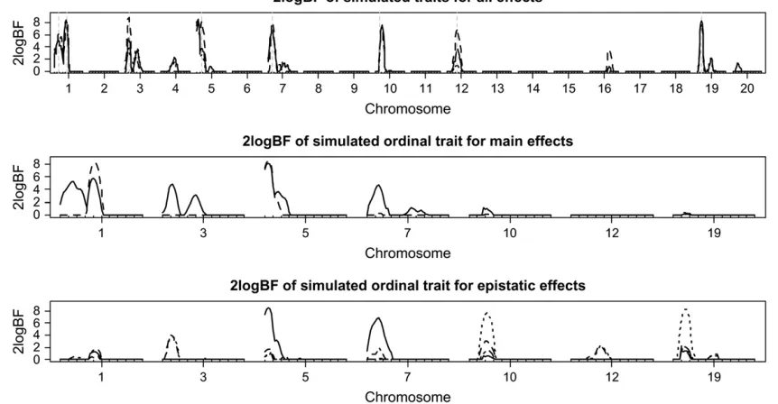
The top section of Figure 5 displays the one-dimen-sional profiles of Bayes factors comparing the model with and without the locus. For the first two analyses, all
the simulated QTL were detected (i.e., 2 logeBF.2.1)
and most of the simulated QTL positions were esti-mated close to the true values. The third analysis, which ignored the property of ordinal traits, missed the weakest QTL on chromosome 12. For chromosome 3, all three analyses detected two peaks, probably resulting from the random error of the simulated data. Among the three analyses, the analysis with the underlying continuous phenotype had the highest Bayes factors for all the detected QTL, followed by the ordinal probit
TABLE 1
F2simulation with eight QTL and two covariates
QTL Chromosome Position Main effect QTL 2 Epistasis
1 1 15 a¼0.5 (0.05)
2 1 45 a¼0.4 (0.03)
d¼0.7 (0.05)
3 3 12 a¼ 0.5 (0.05)
4 5 15 a¼0.5 (0.05)
d¼ 0.5 (0.02)
5 7 15 a¼0.4 (0.03)
5 7 15 4 aa¼ 0.7 (0.04)
6 10 15 8 ad¼1.0 (0.05)
7 12 35 3 da¼0.8 (0.03)
8 19 15
Effects were supplied while heritabilities in parentheses were estimated from a simulated sample of 500 in-dividuals. The effectsa,d,aa,ad, anddarepresent additive, dominance, additive–additive, additive–dominance and dominance–additive effects, respectively. QTL 2 refers to a QTL number.
Figure5.—Simulated F2data analyses: one-dimensional profiles of Bayes factors (rescaled as 2 logeBF and negative values are
model analysis. As expected, the analysis treating the ordinal phenotype as a continuous trait produced the lowest Bayes factors.
For the ordinal probit model analysis, the middle and bottom sections of Figure 5 depict the profiles of Bayes factors for each of the effects comparing models with and without the effect, for the chromosomes with evidence of QTL. These profiles show that our analysis recovered the true genetic effects that influenced the variation of the simulated trait. The estimates of main and epistatic effects for the detected QTL were also close to the true values (not shown here). To investigate which pairs of loci interacted, Figure 6 displays a two-dimensional profile of Bayes factors on the selected chromosomes showing evidence of epistatic QTL. Once again, our analysis recovered the true pattern of epistatic interactions.
DISCUSSION
Yi(2004) proposed a unified Bayesian model
selec-tion framework to identify multiple QTL for complex traits in experimental designs, based upon a composite space representation of the problem. The composite model space approach places a global constraint on the number of detectable QTL and employs latent binary variables to indicate which effects of putative QTL are included in or excluded from the model. The key feature of the composite model space framework is that it provides a convenient framework to reasonably re-duce the model space and to construct efficient MCMC
algorithms. Yi et al. (2005) extended the composite
model space approach to genomewide epistatic QTL analysis for continuous traits and developed efficient MCMC algorithms to explore the posterior distribution. In this study, we extend the composite model space approach to detect multiple interacting QTL for ordinal traits on the basis of a threshold model. Although the threshold model has been widely used in QTL mapping for binary and ordinal traits, few studies address the problem of interacting QTL. Even for continuous traits, it is not a trivial task to extend the existing methods of noninteracting QTL to genomewide interacting-QTL analysis, mainly due to the dramatic increase in the size of model space. Recently, Liet al. (2006) developed a
non-Bayesian method for mapping multiple epistatic QTL for ordinal traits on the basis of the MIM method of Kao et al. (1999) and the threshold model. Our
method is Bayesian implemented via MCMC algorithms whereas MIM uses a maximum-likelihood method to estimate the parameters and a stepwise search pro-cedure to build the model. One of the advantages of the Bayesian approach is that it can simultaneously address both model and parameter uncertainty (Rafteryet al.
1997; Chipmanet al.2001).
Our ordinal probit model simultaneously fits all unknown elements that can potentially influence phe-notypic variation, including arbitrary covariates, main effects of multiple QTL, and gene–gene interactions. We have developed an efficient and easily implemented MCMC algorithm for exploring the posterior of un-knowns in the ordinal probit model. The key idea of our method is that conditional on the latent continuous data, the model becomes the multiple-interacting QTL model for continuous traits and thus the MCMC steps for searching for QTL in Yiet al.(2005) can be used.
Using the real data sets illustrated in this article and extensive simulations (not shown here), the proposed MCMC algorithm was shown to mix rapidly, thus ensur-ing that high-probability models are visited frequently and quickly. The method described herein has been implemented in the package qtlbim for the open-source R environment. Our Bayesian methods developed in this study and other studies, along with the freely available package qtlbim, will greatly facilitate the general usage of the Bayesian methodology for genomewide interact-ing QTL analysis for continuous, binary, and ordinal traits in experimental crosses (Yandellet al.2007).
Several issues deserve further investigation. Corre-lated ordinal and continuous traits are encountered in many QTL studies. Joint analysis of multivariate traits can usually improve statistical power in the detection of QTL and can provide formal procedures to investigate the genetic mechanisms such as pleiotropy and close linkage ( Jiang and Zeng 1995). The data
augmenta-tion approach described herein may be especially attractive for joint analysis of multiple continuous and ordinal traits, where calculating the likelihood can be Figure 6.—Simulated F
2 data analysis with the ordinal
probit model: two-dimensional profiles of Bayes factors (re-scaled as 2 logeBF and negative values are truncated as zero)
difficult. Our future plans also include extensions to experimental crosses derived from multiple inbred lines and outbred populations. More flexible and powerful models for genomewide interacting-QTL analysis are planned. We are also investigating ways to interpret epistasis detected on the basis of the ordinal probit model and to check the fit of inferred QTL models to data and prior assumptions.
This work was supported in part by National Institutes of Health grants R01 GM069430 (N.Y. and B.S.Y.), HL080812 (N.Y.), National Institute of Diabetes and Digestive and Kidney Diseases (NIDDK) 5803701 (B.S.Y.), and NIDDK 66369-01 (B.S.Y.).
LITERATURE CITED
Albert, J. H., and S. Chib, 1993 Bayesian analysis of binary and
polychotomous response data. J. Am. Stat. Assoc.88:669–679. Baierl, A., M. Bogdan, F. Frommletand A. Futschik, 2006 On
lo-cating multiple interacting quantitative trait loci in intercross de-signs. Genetics173:1693–1703.
Ball, R. D., 2001 Bayesian methods for quantitative trait loci
map-ping based on model selection: approximate analysis using the Bayesian information criterion. Genetics159:1351–1364. Bogdan, M., J. K. Ghoshand R. W. Doerge, 2004 Modifying the
Schwarz Bayesian information criterion to locate multiple inter-acting quantitative trait loci. Genetics167:989–999.
Broman, K. W., H. Wu, S´. Senand G. A. Churchill, 2003 R/qtl: QTL
mapping in experimental crosses. Bioinformatics19:889–890. Carlborg, O¨ ., L. Anderssonand B. Kinghorn, 2000 The use of a
genetic algorithm for simultaneous mapping of multiple inter-acting quantitative trait loci. Genetics155:2003–2010. Chen, M. H., and D. K. Dey, 2000 Bayesian analysis for correlated
ordinal data models, pp. 135–162 inGeneralized Linear Models: A Bayesian Perspective, edited by D. K. Dey, S. K. Ghoshand
B. K. Mallick. Marcel Dekker, New York.
Chipman, H., 2004 Prior distributions for Bayesian analysis of
screening experiments, pp. 235–267 inScreening: Methods for Ex-perimentation in Industry, Drug Discovery, and Genetics, edited by A. Deanand S. M. Lewis. Springer, New York.
Chipman, H., E. I. Edwardsand R. E. McCulloch, 2001 The
prac-tical implementation of Bayesian model selection, pp. 65–116 in
Model Selection, edited by P. Lahiri. Beachwood, OH.
Coffman, C. J., R. W. Doerge, K. L. Simonson, K. M. Nichols, C. K.
Duarteet al., 2005 Model selection in binary trait locus
map-ping. Genetics170:1281–1297.
Gelman, A., and D. B. Rubin, 1992 Inference from iterative
simula-tion using multiple sequences (with discussion). Stat. Sci.7:457–511. Gelman, A., J. B. Carlin, H. S. Sternand D. B. Rubin, 2003
Bayes-ian Data Analysis.Chapman & Hall, London.
Hackett, C. A., and J. I. Weller, 1995 Genetic mapping of
quan-titative trait loci for traits with ordinal distributions. Biometrics
51:1252–1263.
Jiang, C., and Z-B. Zeng, 1995 Multiple trait analysis of genetic
map-ping for quantitative trait loci. Genetics140:1111–1127.
Johnson, V. E., and J. H. Albert, 1999 Ordinal Data Modeling.
Springer, New York.
Kao, C. H., and Z-B. Zeng, 2002 Modeling epistasis of quantitative
trait loci using Cockerham’s model. Genetics160:1243–1261. Kao, C. H., Z-B. Zengand R. D. Teasdale, 1999 Multiple interval
mapping for quantitative trait loci. Genetics152:1203–1216. Kass, R. E., and A. E. Raftery, 1995 Bayes factors. J. Am. Stat. Assoc.
90:773–795.
Li, J., S. Wangand Z-B. Zeng, 2006 Multiple interval mapping for
ordinal traits. Genetics173:1649–1663.
Lynch, M., and B. Walsh, 1998 Genetics and Analysis of Quantitative
Traits.Sinauer Associates, Sunderland, MA.
Plummer, M., N. Best, K. Cowlesand K. Vines, 2004 Output Analysis
and Diagnostics for MCMC, v. 0.9–5. (http://www-fis.iarc.fr/coda/). Raftery, A. E., D. Madigan and J. A. Hoeting, 1997 Bayesian
model averaging for linear regression models. J. Am. Stat. Assoc.
92:179–191.
Rao, S., and S. Xu, 1998 Mapping quantitative trait loci for ordered
categorical traits in four-way crosses. Heredity81:214–224. Reifsnyder, P. R., G. Churchilland E. H. Leiter, 2000 Maternal
environment and genotype interact to establish diabesity in mice. Genome Res.10:1568–1578.
Rocha, J. L., E. J. Eisen, F. Seiwerdt, L. D. V. Vleckand D. Pomp,
2004 A large-sample QTL study in mice: III. Reproduction. Mamm. Genome15:878–886.
Sen, S´., and G. Churchill, 2001 A statistical framework for
quan-titative trait mapping. Genetics159:371–387.
Sillanpa¨ a¨, M. J., and J. Corander, 2002 Model choice in gene
map-ping: what and why. Trends Genet.18:301–307.
Wright, S., 1934 An analysis of variability in number of digits in an
inbred strain of guinea pigs. Genetics19:506–536.
Xu, S., and W. R. Atchley, 1996 Mapping quantitative trait loci for
complex binary diseases using line crosses. Genetics143:1417– 1424.
Xu, C., Y.-M. Zhangand S. Xu, 2005 An EM algorithm for mapping
quantitative resistance loci. Heredity94:119–128.
Xu, S., N. Yi, D. Burke, A. Galekiand R. A. Miller, 2003 An EM
algorithm for mapping binary disease loci: application to fibro-sarcoma in a four-way cross mouse family. Genet. Res.82:127– 138.
Yandell, B. S., T. Mehta, S. Banerjee, D. Shriner, R. Venkataraman
et al., 2007 R/qtlbim: QTL with Bayesian interval mapping in ex-perimental crosses. Bioinformatics23:641–643.
Yi, N., 2004 A unified Markov chain Monte Carlo framework for
mapping multiple quantitative trait loci. Genetics167:967–975. Yi, N., and S. Xu, 2000 Bayesian mapping of quantitative trait loci
for complex binary traits. Genetics155:1391–1403.
Yi, N., S. Xu, V. Georgeand D. B. Allison, 2004 Mapping multiple
quantitative trait loci for complex ordinal traits. Behav. Genet.
34:3–15.
Yi, N., B. S. Yandell, G. A. Churchill, D. B. Allison, E. J. Eisenet al.,
2005 Bayesian model selection for genome-wide epistatic quan-titative trait loci analysis. Genetics170:1333–1344.
Zeng, Z-B., 1994 Precision mapping of quantitative trait loci. Genetics
136:1457–1468.
Zeng, Z-B., T. Wangand W. Zou, 2005 Modeling quantitative trait
loci and interpretation of models. Genetics169:1711–1725.