Multinuclear Solid-State Nuclear Magnetic Resonance Spectroscopy of Microporous Materials

(1)

Scholarship@Western

Electronic Thesis and Dissertation Repository

12-12-2013 12:00 AM

Multinuclear Solid-State Nuclear Magnetic Resonance

Spectroscopy of Microporous Materials

Jun Xu

The University of Western Ontario Supervisor

Yining Huang

The University of Western Ontario Graduate Program in Chemistry

A thesis submitted in partial fulfillment of the requirements for the degree in Doctor of Philosophy

Follow this and additional works at: https://ir.lib.uwo.ca/etd

Part of the Inorganic Chemistry Commons

Recommended Citation Recommended Citation

Xu, Jun, "Multinuclear Solid-State Nuclear Magnetic Resonance Spectroscopy of Microporous Materials" (2013). Electronic Thesis and Dissertation Repository. 1752.

https://ir.lib.uwo.ca/etd/1752

This Dissertation/Thesis is brought to you for free and open access by Scholarship@Western. It has been accepted for inclusion in Electronic Thesis and Dissertation Repository by an authorized administrator of

(2)

(Thesis format: Integrated Article)

by

Jun Xu

Graduate Program in Chemistry

A thesis submitted in partial fulfillment of the requirements for the degree of

Doctor of Philosophy

The School of Graduate and Postdoctoral Studies The University of Western Ontario

London, Ontario, Canada

(3)

Abstract

Microporous materials have attracted tremendous attention since the 18th century due

to their industrial importance in the broad areas of ion exchange, catalysis, adsorption, etc. It

is essential to understand the relationships between the properties of microporous materials

and their structures. However, the structures of many microporous materials are determined

from the more limited powder X-ray diffraction (XRD) data due to the lack of suitable

single-crystals for XRD. In such cases, an unambiguous structure solution of microporous

materials requires additional information from other techniques such as solid-state NMR

(SSNMR) spectroscopy. SSNMR spectroscopy can provide short-range information around

the NMR-active nucleus of interest and it can also confirm the long-range ordering of the

structure such as crystal symmetry. This thesis is focused on the study of two types of

microporous materials, metal–organic frameworks (MOFs) and titanosilicates, by

multinuclear SSNMR spectroscopy in combination with quantum chemical calculations for

computational modeling.

A brief introduction is first given in Chapter 1. In Chapter2–6, multinuclear SSNMR

investigations of two prototypical MOFs with potential industrial applications, CPO-27-M

(M = Mg, Zn, Co, Ni), and α-Mg3(HCOO)6, are carried out. MOFs are novel

inorganic-organic hybrid microporous materials, constructed by the interconnection of metal ions by

various organic linkers. MOFs have many promising properties compared to classical

microporous materials such as rich structural diversity, high thermal stability, tunable

porosity, selective adsorption, etc. The results presented in these chapters demonstrate that

SSNMR spectroscopy is very suitable for the characterization of MOFs: The local Mg

environments and the rehydration/adsorption processes of CPO-27-Mg were examined by

natural abundance 25Mg SSNMR spectroscopy at an ultrahigh magnetic field of 21.1 T. The

dynamics of several guest molecules inside of CPO-27-M were monitored by

variable-temperature 2H SSNMR spectroscopy. The structures of another MOF, α-Mg3(HCOO)6,

before and after guest adsorption, were thoroughly investigated by 1H, 2H, 13C, 17O, and 25Mg

SSNMR spectroscopy. Moreover, the existence of weak C–H⋅⋅⋅O and C–H⋅⋅⋅N hydrogen

bonding were confirmed by ultrahigh-resolution 1H SSNMR spectroscopy.

(4)

and 47/49Ti SSNMR spectroscopy. Microporous titanosilicates are novel inorganic materials

with many unique structural features. This work is highlighted by the acquisition of natural

abundance SSNMR spectra for three unreceptive quadrupolar nuclei, 47/49Ti and 39K, at 21.1

T. 47/49Ti SSNMR experiments provides insights into the coordination environments of Ti

inside the framework, whereas 39K SSNMR experiments allow one to directly probe the local

environment of extra-framework counter cations in titanosilicates.

Keywords

Metal–organic frameworks, titanosilicates, structure characterization, solid-state NMR,

unreceptive quadrupolar nuclei, ultrahigh field, adsorption, guest dynamics.

(5)

Co-Authorship Statement

This thesis contains materials from previously published manuscripts. Dr. Yining

Huang was the corresponding author on all the presented papers and was responsible for the

supervision of Jun Xu over the course of his Ph.D. study. For copyright releases see the

Appendix.

Chapter 2 is from the published letter co-authored by Jun Xu, Victor V. Terskikh and

Yining Huang (J. Phys. Chem. Lett. 2013, 4, 7-11). The samples were prepared by J. Xu.

Experiments were performed by J. Xu and V. V. Terskikh. J. Xu wrote the manuscript. V. V.

Terskikh and Y. Huang revised the manuscript.

The majority of Chapter 3 is from the published communication co-authored by Jun

Xu, Victor V. Terskikh and Yining Huang (Chem. Eur. J. 2013, 19, 4432-4436). J. Xu

prepared the samples. J. Xu and V. V. Terskikh performed experiments. The manuscript was

written by J. Xu and it was revised by V. V. Terskikh and Y. Huang.

Dr. Victor V. Terskikh is credited for the acquisition of SSNMR spectra presented in

Chapter 4. Theoretical calculations were also performed by V. V. Terskikh.

Regina Sinelnikov is thanked for making CPO-27-M samples used in Chapter 5.

Chapter 6 is a portion of the published article co-authored by Peng He, Jun Xu,

Victor V. Terskikh, Andre Sutrisno, Heng-Yong Nie and Yining Huang (J. Phys. Chem. C

2013, 117, 16953-16960). The samples were provided by P. He and J. Xu. 17O NMR spectra

were collected by J. Xu and V. V. Terskikh. A. Sutrisno is credited and thanked for analyzing

17

O NMR spectra. 17O contents of the samples were measured by H.-Y. Nie. Y. Huang was

responsible for writing and editing the drafts. P. He, J. Xu, V. V. Terskikh and A. Sutrisno

revised the manuscript.

Dr. Zhi Lin (University of Aveiro, Portugal) is credited for preparing the TiSiO4

samples used in Chapter 7. Dr. Victor V. Terskikh is thanked for the acquisition of 47/49Ti

and 39K SSNMR spectra shown in Chapter 7. Theoretical calculations were also conducted

by V. V. Terskikh.

(6)

Acknowledgments

First and foremost, without any doubt, I would like to express the deepest gratitude to

my advisor, Dr. Yining Huang, for all I have learned from him. I would also like to thank

him for tolerating, encouraging and helping me to shape my interest and ideas. Without his

supervision and constant help this dissertation would not have been possible.

Then I would like to thank the members of my thesis examination board: Dr. Zhifeng

Ding, Dr. Johanna M. Blacquiere, Dr. John R. de Bruyn (Department of Physics and

Astronomy) and Dr. Luis Smith (Clark University, USA). The examiners of my first year

report are also thanked: Dr. Yang Song, Dr. Nicholas C. Payne, Dr. Melvyn C. Usselman and

Dr. Heinz-Bernhard Kraatz. I would like to express my gratitude to Dr. Yang Song, Dr.

Victor N. Staroverov, Dr. Nicholas C. Payne and Dr. Lyudmila Goncharova (Department of

Physics and Astronomy) for giving their interesting courses during my graduate studies,

which were very helpful and valuable. I would like to specially thank Dr. Mathew Willans

for his technical help and thoughtful comments on any problem with the NMR spectrometer.

I would also thank Dr. Paul Boyle for single-crystal XRD experiments and Dr. Doug

Hairsine for mass spectrometer analysis. Thanks for graduate coordinator Ms. Darlene

McDonald, administrative minister Ms. Anna Vandendries-Barr, departmental secretaries Ms.

Sandy McCow and Ms. Clara Fernandes for their help during my Ph.D. program. I would

like to thank departmental manager Mr. Warren Lindsay and electronics shop staffs Mr. John

Vanstone and Mr. Barakat Misk for their technical supports. Mr. Yves Rambour in glass

blowing shop is credited as well for the glass blowing course and his help during the past five

years. I would thank lab technicians Ms. Lesley Tchorek, Ms. Susan England, Ms. Sandra Z.

Holtslag and Mr. Robert Harbottle for helping me to finish the teaching assistant duties. In

addition, I would like to thank Ms. Kim Law and Ms. Grace Yau in Department of Earth

Sciences for powder XRD experiments and Dr. Heng-Yong Nie in Surface Science Western

for measuring the 17O contents. I would like to express my sincere gratitude to Dr. Victor V.

Terskikh at the National Ultrahigh-field NMR Facility for Solids for acquiring NMR spectra

at 21.1 T and providing NMR technical assistance during my visit to Ottawa. He is also

credited for performing CASTEP theoretical calculations. I would like to thank Dr. Luke

O’Dell (Deakin University, Australia) for providing the EXPRESS simulation package, Dr.

(7)

SHARCNET (Shared Hierarchical Academic Research Computing Network) facilities for

computational resources, and Dr. David L. Bryce (University of Ottawa) for the EFGShield

program. I thank Dr. Zhi Lin (University of Aveiro, Portugal) for providing titanosilicate

samples. Dr. Song Yang and Dr. Kim M. Baines are thanked for the access of glove boxes.

The financial support from Department of Chemistry is also gratefully acknowledged.

Moreover, I would like to extend my gratitude to my past and present colleagues: Dr.

Zhimin (Steven) Yan, Janice A. Lee, Yueqiao (Rachel) Fu, Dr. Andre Sutrisno, Dr. Lu Zhang,

Dr. Margaret Hanson, Dr. Li Liu, Tetyana Levchenko, Adam Macintosh, Donghan Chen,

Yue Hu, Zheng (Sonia) Lin, Le Xu, Peng He, Maxwell Goldman, Dr. Wei (David) Wang, Dr.

Haiyan Mao, Dr. Farhana Gul-E-Noor, Yuanjun Lu, Shoushun Chen and Regina Sinelnikov.

The patience, enthusiasm, humor, optimism and collaboration from them will accompany me

for all my life.

Finally and most importantly, I would like to express my deepest gratitude to my

family (my parents, my sister and my cute niece). Without their continuous love, support and

encouragement I would not be able to finish my Ph. D. program, especially during tough

times.

(8)

List of Tables

Table 1-1: The guideline to predict the nuclear spin. ... 9

Table 1-2: Typical magnitudes of nuclear spin interactions (Ref. 8). ... 10

Table 1-3: Nuclear properties of nuclei studied in this thesis. ... 21

Table 3-1: Experimental and calculated 25Mg NMR parameters. ... 73

Table 4-1: Experimental and calculated 1H and 13C isotropic chemical shifts. ... 97

Table 4-2: Experimental and calculated 13C CSA tensors. ... 100

Table 4-3: Experimental and calculated 25Mg NMR parameters of the pyridine sample. .... 114

Table 5-1: Simulated 2H NMR parameters and motions. ... 162

Table 6-1: Experimental 17O NMR parameters of the MOF samples. ... 181

Table 7-1: Experimental 49Ti NMR parameters. ... 222

(14)

List of Figures

Figure 1-1: The structure of zeolite Y viewed down [110] direction. The bridge oxygens are

omitted for clarity. ... 2

Figure 1-2: Some unique structural features of TiSiO4 compared to zeolites. ... 2

Figure 1-3: The structures of IRMOF series. (Ref. 19) ... 3

Figure 1-4: Schematic diagram of the solvothermal synthesis of α-Mg3(HCOO)6. ... 4

Figure 1-5: Schematic illustration of Bragg’s Law... 5

Figure 1-6: Schematic illustration of Zeeman’s energy levels that appear for spin-3/2 nucleus placed into the external magnetic filed B0. ... 11

Figure 1-7: Left: ellipsoid representation of the chemical shielding tensor, whose principle axes coincide with the chemical shielding tensor principle axis system and the length of each principle axis of which is proportional to the principle value of the shielding tensor associated with that principle axis. Right: analytical simulations (performed using DMFIT software) of theoretical 13C CSA powder patterns (δiso = 0 ppm). Ω is set to 0 ppm for the top spectrum while it is 200 ppm for the other spectra. ... 13

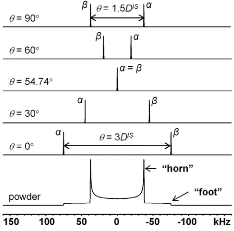
Figure 1-8: Analytical simulations (performed using DMFIT software) of theoretical 1H–1H homonuclear dipolar coupling powder patterns. DIS is set to 50 kHz. For heteronuclear dipolar coupling, the doublet splitting is DIS at 90° and 2DIS at 0°. ... 16

Figure 1-9: Charge distribution in (a) spin-1/2 nuclei and (b) quadrupolar nuclei. ... 17

Figure 1-10: Energy level diagram of a spin-5/2 nucleus, showing how the splitting due to the Zeeman interaction is perturbed to first- and second-order by the quadrupolar interaction. (Ref. 34) ... 19

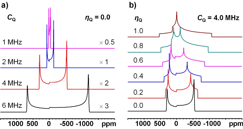
Figure 1-11: Analytical simulations (performed using DMFIT software) of theoretical 25Mg

(I = 5/2) powder patterns of the CT (ν0 = 24.5 MHz, δiso = 0 ppm) at 9.4 T, broadened by the

(15)

η

and shape are also illustrated. ... 20

Figure 1-12: (a) Schematic diagram of the magic-angle spinning (MAS) experiment.

Analytical simulations (performed using DMFIT software) of (b) theoretical 13C (I = 1/2, ν0 =

100.6 MHz) CSA patterns and (c) 25Mg (I = 5/2, ν0 = 24.5 MHz) quadrupolar patterns of the

CT at 9.4 T, under MAS and static conditions. ... 23

Figure 1-13: Pulse sequence for cross-polarization from abundant spin I to dilute spin S with

detection of the S magnetization. τ is the contact time. ... 24

Figure 1-14: Plot of the CP signal intensity as a function of the contact time τ. ... 25

Figure 1-15: Pulse sequence for 1H–13C FSLG-HETCOR. θm is the magic-angle pulse

(54.74°). ... 26

Figure 1-16: (a) The QCPMG pulse sequence. The block inside the brackets is called a

Meiboom-Gill (MG) loop and it is repeated for N times. (b) An example of FID and

spectrum of the QCPMG experiment. ... 27

Figure 1-17: (a) Pulse sequence of BABA DQ MAS experiment. N is the number of rotor

cycles used for excitation and reconversion. (b) Schematic representation of the typical

pattern observed in 2D DQ MAS spectrum (Ref. 32). AA and BB are correlation peaks from

two like spins while AB is from two unlike spins. ... 30

Figure 1-18: (a) Comparison of calculated (solid line) and experimentally (data points)

observed DQ signal intensities. The experiments were performed on tribromoacetic acid,

which is a 1H–1H spin pair model compound with a dipolar coupling of DIS = 2π× 6.5 kHz.

IDQ is normalized with respect to the signal of a one-pulse experiment. (b) Simulated DQ

build-up curves for different spin systems (solid lines). The three, four, and six spins are

localized at the vertices of an equilateral triangle, a square, a tetrahedron, and an octahedron,

respectively. IDQ is normalized to the number of coupled pairs in the respective system, and

the dashed lines indicate the long-time limit for DQ intensities, provided that only two-spin

DQ coherences are excited. The two figures are taken from Ref. 32. The dashed line in (a) or

(16)

the dotted line in (b) is the leading two-spin term (IDQ∝ (D ) τexc ) in the series expansion

for multispin systems. ... 31

Figure 1-19: An example of 2D 3QMAS spectrum (a) before and (b) after shearing. ... 32

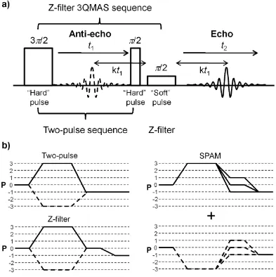
Figure 1-20: (a) The pulse sequence of 3QMAS experiment. (b) The coherence transfer

pathway of the two-pulse, Z-filter, and SPAM-3QMAS. The solid line is the echo pathway

while the dashed line is the anti-echo pathway. P is the coherence order. ... 33

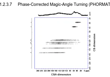
Figure 1-21: The 1H-13C PHORMAT 2D spectrum of tyrosine⋅HCl (Ref. 73). ... 35

Figure 1-22: (a) Energy level diagram of 2H (I = 1), showing how the splitting due to the

Zeeman interaction is perturbed to first-order by the quadrupolar interaction. (b) Schematic

illustration of the formation of a static 2H powder pattern with a typical Pake doublet (ηQ = 0).

The doublet is due to the two allowed transitions... 36

Figure 1-23: Analytical simulations (performed using EXPRESS software, CQ = 155 kHz, ηQ

= 0.0) of theoretical 2H powder patterns for (a) different motions in the fast-limit regime, and

(b) in-plane rotation of C6D6 about its C6 axis (referred to as C6) as a function of rate constant.

The motions in (a) are C1 rotation about C–2H bond (referred to as C1), flip-flop of

benzene-d4 about its C2 axis (referred to as C2), methyl C–2H rotation about its C3 axis (referred to as

C3), and the three deuterated methyl groups of t-butyl rotate about their C3 axes while the t

-butyl group as a whole also rotate about its C3’ axis (referred to as C3 + C3’). ... 38

Figure 2-1: The reversible transformation of a local Mg environment in CPO-27-Mg. For

clarity, the hydrogens of water in the channels are omitted. ... 47

Figure 2-2: 25Mg static SSNMR spectra of CPO-27-Mg as a function of rehydration degree.

All spectra were acquired under the same spectrometer conditions, 16384 scans and a pulse

delay of 1 s. The * indicates a small amount of impurity. ... 51

Figure 2-3: The plot of calculated (a) CQ(25Mg) and (b) δiso(25Mg) as a function of the Mg–

OH2 distance. ... 54

(17)

All spectra were acquired under the same spectrometer conditions, 16384 scans and a pulse

delay of 1 s. ... 55

Figure 2-5: The plot of calculated (a) CQ(25Mg) and (b) δiso(25Mg) as a function of the Mg–

OC(CH3)2 distance. ... 56

Figure 3-1: The framework and Mg coordination environments of the DMF sample.

Hydrogen atoms of the encapsulated DMF are omitted for clarity. ... 68

Figure 3-2: (a) Natural abundance 25Mg static, and (b) 5 kHz MAS spectra of four

microporous α-Mg3(HCOO)6 phases at 21.1 T. *: spinning sidebands. ... 69

Figure 3-3: Natural abundance 25Mg SPAM-3QMAS spectrum of the activated sample. The

dashed lines correspond to the slices taken for simulation. The MAS spectrum simulated with

the parameters obtained from 3QMAS is also shown. ... 70

Figure 3-4: Natural abundance 25Mg SPAM-3QMAS spectrum of the DMF sample. The

Figure 3-5: Natural abundance 25Mg SPAM-3QMAS spectrum of the acetone sample. The

Figure 3-6: Natural abundance 25Mg SPAM-3QMAS spectrum of the benzene sample. The

Figure 4-1: Left: The framework of the DMF phase. Right: Chemical environments of H, C

and Mg. Hydrogen atoms of the encapsulated DMF are omitted for clarity. ... 90

Figure 4-2: Illustration of the enhancement of 1H spectral resolution for the activated sample

by: (a) MAS and (b) MAS combined with the isotopic dilution. *: residual DMF signal. .... 91

(18)

Figure 4-3: Experimental and deconvoluted 62.5 kHz MAS (a) H and (b) 18 kHz H→ C

CPMAS (with a contact time of 2 ms) spectra of the 20% H α-Mg3(HCOO)6 samples. The

protons labeled with red color exhibit significant guest-induced shifts while the protons and

carbons labeled with blue color were only tentatively assigned. ... 93

Figure 4-4: 2D 1H–1H BABA DQ spectra of the 20% H activated sample as a function of

excitation time (spinning speed: 18 kHz). Diagonals (dash lines) are drawn to illustrate the

self-correlation peaks while horizontal lines (labeled in red) indicate the cross peaks. Only

new correlations are shown at longer excitation time for clarity. Three spectra have the same

contour levels. The neighboring protons around H2 are shown at top right. ... 95

Figure 4-5: 2D 1H–13C FSLG-HETCOR spectrum (contact time: 35 μs) of the 20% H

activated sample (spinning speed: 18 kHz). The dashed lines indicate the direct bonding

between 1H and 13C. The 62.5 kHz MAS 1H spectrum was used as the projection along the

indirect (1H) dimension. ... 98

Figure 4-6: 2D 1H-13C PHORMAT spectrum of the 100% H activated sample (spinning

speed: 2 kHz). The dashed lines correspond to the slices taken for simulation... 99

Figure 4-7: 2D 1H–1H BABA DQ spectra of the 20% H DMF sample as a function of

excitation time (spinning speed: 18 kHz). Three DQ spectra were set to have the same

contour levels. Bottom right: 2D 1H–13C FSLG-HETCOR spectrum (contact time 35 μs) of

the 20% H DMF sample (spinning speed: 18 kHz). The 62.5 kHz MAS 1H spectrum was

used as the projection along the indirect (1H) dimension. ... 102

Figure 4-8: 2D 1H–1H BABA DQ spectra of the 20% H benzene sample as a function of

the 20% H benzene sample (spinning speed: 18 kHz). The 62.5 kHz MAS 1H spectrum was

Figure 4-9: 2D 1H–1H BABA DQ spectra of the 20% H acetone sample as a function of

(19)

Figure 4-10: 2D 1H–13C PHORMAT spectra of the 100% H DMF and benzene samples

(spinning speed: 2 kHz). ... 105

Figure 4-11: Local environments around (a) DMF and (b) benzene. For benzene, the induced

magnetic field is shown to visualize the ring current effect. ... 107

Figure 4-12: (a): 1H→13C CPMAS spectra (contact time: 2 ms) of the 20% H benzene sample

as a function of spinning speed. Simulated spinning sideband patterns of benzene are shown.

(b): Room temperature 2H static spectrum of α-Mg3(HCOO)6⊃C6D6 at 9.4 T. ... 108

Figure 4-13: Room temperature 2H static spectrum of α-Mg3(HCOO)6⊃pyridine-d5 at 9.4 T.

*: additional motions... 109

Figure 4-14: 2D 1H–1H BABA DQ spectra of the 20% H pyridine sample as a function of

the 20% H pyridine sample (spinning speed: 18 kHz). The 62.5 kHz MAS 1H spectrum was

used as the projection along the indirect (1H) dimension. The protons and carbons labeled

with blue color were only tentatively assigned. ... 111

Figure 4-15: Natural abundance (a) static, (b) 5 kHz MAS, and (c) 2D SPAM-3QMAS 25Mg

spectra of the 20% H pyridine sample. The static and MAS spectra simulated with the

parameters obtained from 3QMAS are also shown. All 25Mg NMR experiments were

performed at 21.1 T... 113

Figure 5-1: Left: The channels of dehydrated CPO-27-M. Right: The local environments of

M2+ in as-made and dehydrated (activated) CPO-27-M. ... 127

Figure 5-2: Schematic illustration of guest dynamics using D2O adsorbed on CPO-27-M as

an example: (a) π flip-flop of D2O about its C2 axis (i.e., internal motion) followed by (b)

uniaxial rotation of the whole D2O molecule (i.e., external motion). ϕ is the angle between

the Z axis of the intermediate frame (C2 axis of D2O) and the rotation axis. ... 133

(20)

the a,b plane. (b) In the language of NMR, the hopping of a guest molecule between different

M2+ ions in the a,b plane are equivalent to motions occurring on the base of a cone with the

cone angle of θ. (c) Analytical simulations (performed using EXPRESS package) of 2H static

powder patterns of multiple-site hopping in the fast-limit regime. ... 135

Figure 5-4: Experimental 2H static spectra of D2O in CPO-27-Mg at 293 K as a function of

loading... 136

Figure 5-5: Experimental and simulated 2H static spectra of the 0.6D2O/Mg sample as a

function of temperature. The dynamic model for simulation: π flip-flop of D2O about its C2

axis. ... 138

Figure 5-6: Experimental 2H static spectra of (a) D2O in CPO-27-Zn at 293 K as a function of

loading, and (b) the 0.6D2O/Zn sample as a function of temperature. ... 139

Figure 5-7: Experimental and simulated 2H static spectra of CD3CN in CPO-27-Mg at 293 K

as a function of loading. The dynamic models for simulation: rotation of methyl C–D about

its C3 axis followed by non-localized six-site (or two-site) hopping motions. ... 140

Figure 5-8: Schematic illustration of the local geometry of CD3CN adsorbed in CPO-27-M as

a function of loading. ... 141

Figure 5-9: Experimental 2H static spectra of the 0.6CD3CN/Mg sample as a function of

temperature. The dynamic models for simulation: rotation of methyl C–2H about its C3 axis

followed by non-localized six-site (or two-site) hopping motions. ... 142

Figure 5-10: A detailed schematic illustration of the non-localized multiple-site hopping

viewed along the c axis (left) and perpendicular to the c axis (right). ... 143

Figure 5-11: Experimental and simulated 2H static spectra of the 0.4CD3CN/Zn sample as a

function of temperature. The dynamic models for simulation: rotation of methyl C–2H about

(21)

293 K as a function of loading. The dynamic models for simulation: rotation of methyl C–2H

about its C3 axis followed by non-localized six-site (or two-site) hopping motions. ... 147

Figure 5-13: Schematic illustration of the local geometry of acetone-d6 adsorbed in

CPO-27-M as a function of loading. ... 148

Figure 5-14: Experimental and simulated 2H static spectra of the 0.6(CD3)2CO/Mg sample as

a function of temperature. The dynamic models for simulation: rotation of methyl C–D about

Figure 5-15: Arrhenius plot for the rate constant of the two-site hopping motion between 193

and 143 K. ... 150

Figure 5-16: Experimental and simulated 2H static spectra of acetone-d6 in CPO-27-Zn at 293

K as a function of loading. The dynamic models for simulation: rotation of methyl C–D

about its C3 axis followed by non-localized six-site (or two-site) hopping motions of the

whole molecule. ... 151

Figure 5-17: Experimental and simulated 2H static spectra of the 0.2(CD3)2CO/Zn sample as

a function of temperature. The dynamic models for simulation: rotation of methyl C–2H

about its C3 axis followed by non-localized six-site (or three-site) hopping motions. ... 152

Figure 5-18: Experimental and simulated 2H static spectra of the 0.2C6D6/Mg sample as a

function of temperature. The dynamic models for simulation: in-plane rotation of benzene

about its C6 axis followed by non-localized six-site hopping. ... 154

Figure 5-19: Experimental 2H static spectra of C6D6 in CPO-27-Zn at 293 K as a function of

loading... 155

Figure 5-20: Experimental 2H static spectra of the 0.2C6D6/Zn sample as a function of

temperature. The dynamic models for simulation: in-plane rotation of benzene about its C6

axis followed by non-localized six-site hopping. ... 156

(22)

function of temperature. The dynamic models for simulation: in-plane rotation of benzene

about its C6 axis followed by non-localized six-site hopping. ... 158

Figure 5-22: Experimental 2H static spectra of the 0.2C6D6/Co sample as a function of

temperature. ... 160

Figure 6-1: Illustrations of the framework with DMF (solvent) in the pore, Mg, and O

environments of microporous α-Mg3(HCOO)6. The hydrogens of DMF are omitted for

clarity. ... 179

Figure 6-2: Experimental and simulated 17O (a) MAS and (b) static SSNMR spectra of

microporous α-Mg3(HCOO)6 at 21.1 T. *: spinning sidebands. ... 180

Figure 6-3: Illustrations of the framework, Mg and O environments of activated CPO-27-Mg.

... 181

Figure 6-4: Experimental and simulated 17O MAS SSNMR spectra of (a) as-made and (b)

activated CPO-27-Mg at 21.1 T. ◊: 17O background signal from ZrO2 rotor. (Ref. 53) ... 182

Figure 7-1: Left: the structure of natisite (Na–O bonds are omitted for clarity). Right: local

environments of Ti4+ and Na+. The atoms on the blue parallelograms are co-planar. ... 199

Figure 7-2: (a) 29Si MAS spectrum of natisite at 9.4 T. (b) Experimental (QCPMG) and

simulated natural abundance 47/49Ti static spectra of natisite at 21.1 T. (c) Experimental and

simulated 23Na MAS spectra of natisite at 9.4 T (top); 23Na 2D 3QMAS spectrum of natisite

at 9.4 T (bottom). The dashed lines corresponds to the slices taken for simulation (Na(I) only,

since the signal of Na1 was too weak). The simulated 23Na MAS spectrum was based on the

parameters obtained from 3QMAS. *: spinning sidebands. ... 200

Figure 7-3: Left: the structure of AM-1 (The hydrogen atoms and Na–O bonds are omitted

for clarity). Right: 6-rings and local environments of Ti4+ and Na+. The atoms on the blue

parallelograms are co-planar. ... 203

Figure 7-4: (a) 29Si MAS SSNMR spectrum of AM-1 at 9.4 T. #: impurity. (b) Experimental

and simulated 23Na MAS SSNMR spectra of AM-1 at 9.4 T. (c) Experimental (QCPMG) and

(23)

the transmitter frequency is indicated on each sub-spectrum. ... 204

Figure 7-5: Left: the structure of AM-4 (left, the hydrogen atoms and Na–O bonds are

omitted for clarity). Right: brookite-type zigzag TiO6 chains and the local environment of

Ti4+. The Ti–O distances are shown in Å. ... 205

Figure 7-6: (a) Experimental and deconvoluted 29Si MAS spectra of AM-4 at 9.4 T. (b)

Experimental (QCPMG) and simulated natural abundance 47/49Ti static spectra of AM-4 at

21.1 T. The offset of the transmitter frequency is indicated on each sub-spectrum. (c)

Experimental and simulated 23Na MAS spectra of AM-4 at 9.4 T (top); 23Na 2D 3QMAS

spectrum of AM-4 at 9.4 T (bottom). The simulated 23Na MAS spectrum was based on the

parameters obtained from 3QMAS. ... 207

Figure 7-7: Left: the structure of sitinakite. The hydrogen atoms and Na–O bonds are omitted

for clarity. Right: the structure of Ti4O16 cluster. ... 209

Figure 7-8: (a) Experimental 29Si MAS SSNMR spectrum of sitinakite at 9.4 T. (b)

Experimental (Echo) and simulated natural abundance 47/49Ti static SSNMR spectra of

sitinakite at 21.1 T. (c) Experimental and simulated 23Na MAS SSNMR spectra of sitinakite

at 9.4 T (top); 23Na 2D 3QMAS spectrum of sitinakite at 9.4 T (bottom). The simulated 23Na

MAS spectrum was based on the parameters obtained from 3QMAS. ... 210

Figure 7-9: Left: the structure of KGTS-1. The hydrogen atoms and K–O bonds are omitted

for clarity. Right: the local environment of Ti4+. The Ti–O distances of two GTS-1 phases are

shown in Å. ... 212

Figure 7-10: (a) Experimental 29Si MAS SSNMR spectrum of GTS-1 at 9.4 T. (b)

Experimental (Echo and QCPMG) and simulated natural abundance 47/49Ti static SSNMR

spectra of GTS-1 at 21.1 T. The offset of the transmitter frequency is indicated on each

sub-spectrum. ... 213

Figure 7-11: (a) 23Na MAS SSNMR spectra of GTS-1 at 9.4 T as a function of pulse delay

(pd). (b) 23Na 3QMAS spectrum of GTS-1 at 9.4 T (bottom). The dashed lines correspond to

the slices taken for simulation. (c) Experimental and simulated 23Na MAS SSNMR spectra of

(24)

spectrum of (a). (d) Natural abundance 39K MAS SSNMR spectra of GTS-1 at 21.1 T as a

function of pulse delay (pd). (e) Experimental and simulated natural abundance 39K MAS

SSNMR spectra of GTS-1 at 21.1 T. The simulated 39K MAS spectrum was based on the parameters obtained from the difference spectrum of (d). *: spinning sidebands. ◊: transmitter artifact. ... 215

Figure 7-12: The structure of ETS-4. The hydrogen atoms and Na+ cations are omitted for

clarity. ... 217

Figure 7-13: (a) Experimental 29Si MAS SSNMR spectrum of ETS-4 at 9.4 T. (b)

Experimental (Echo) natural abundance 47/49Ti static SSNMR spectrum of ETS-4 at 21.1 T.

(c) Experimental and simulated 23Na MAS SSNMR spectra of ETS-4 at 9.4 T (top); 23Na

3QMAS spectrum of ETS-4 at 9.4 T (bottom). The dashed lines correspond to the slices

taken for simulation. Simulated 23Na MAS spectrum was based on the parameters obtained

from 3QMAS. ... 218

Figure 7-14: The structure of ETS-10. The bridging O atoms are omitted to show the

connectivity between Si/Si and Si/Ti. The distance a ≈ b causes the stacking defaults. The

dashed line presents the TiO6 chains. The five possible Na sites are also shown. ... 219

Figure 7-15: (a) Experimental 29Si MAS SSNMR spectrum of ETS-10 at 9.4 T. (b)

Experimental (Echo) and simulated natural abundance 47/49Ti static SSNMR spectra of

ETS-10 at 21.1 T. (c) Experimental 23Na MAS SSNMR spectrum of ETS-10 at 9.4 T (top); 23Na

3QMAS spectrum of ETS-4 at 9.4 T (bottom). (d) Experimental and simulated 39K MAS

SSNMR spectra of ETS-10 at 21.1 T. *: spinning sidebands. ... 221

(25)

List of Abbreviations

1D one-dimensional

2D two-dimensional

3D three-dimensional

3Q triple-quantum

3QMAS triple-quantum magic-angle spinning

B3LYP Becke’s 3-parameter hybrid density exchange functional with Lee, Yang and

Parr correlation functional

BABA back-to-back

BDC 1, 4-benzenedicarboxylate

Cp cyclopentadienyl

CP cross-polarization

CPMAS cross-polarization magic-angle spinning

CPO Coordination Polymer of Oslo

CS chemical shielding

CSA chemical shielding anisotropy

CT central transition

CW continuous-wave

DAS dynamic-angle spinning

DFS double-frequency sweeps

DFT density functional theory

DMF N,N-dimethylformamide

DOBDC 2,5-dioxido-1,4-benzenedicarboxylate

DOR double-rotation

DQ double-quantum

EDS energy dispersive X-ray spectroscopy

EFG electric field gradient

ETS Engelhard titanosilicate

FID free induction decay

FSLG frequency-switched Lee-Goldberg

(26)

FWHH full-width at half-height

GGA Generalized Gradient Approximation

GIPAW Gauge Including Projector Augmented Wave

GTO Gaussian-type orbital

HB Herzfeld-Berger

HETCOR hetero-nuclear correlation

HTS hydrothermal synthesis

IUPAC International Union of Pure and Applied Chemistry

IRMOF isoreticular metal–organic framework

MAS magic-angle spinning

MAT magic-angle turning

MOF metal–organic framework

MP2 second-order Møller-Plesset perturbation theory

MQ multiple-quantum

MQMAS multiple-quantum magic-angle spinning

N.A. natural abundance

NMR nuclear magnetic resonance

NPD neutron powder diffraction

o.d. outer diameter

PAS principle axis system

PBE Perdew, Burke and Ernzerhof correlation functional

PHORMAT phase-corrected magic-angle turning

ppm parts per million

PXRD powder X-ray diffraction

QCPMG quadrupolar Carr-Purcell-Meiboom-Gill pulse sequence

QE quadrupolar echo

rf radio frequency

S/N signal-to-noise ratio

SEM scanning electron microscopy

SPAM soft-pulse-added-mixing

SQ single-quantum

(27)

SSNMR solid-state nuclear magnetic resonance

STS solvothermal synthesis

SW spectral width

THF tetrahydrofuran

TGA thermogravimetric analysis

TiSiO4 titanosilicate-based materials

TMS tetramethylsilane

TOF-SIMS time-of-flight secondary ion mass spectrometry

TPPM two-pulse phase-modulation

TTMSS tetrakis(trimethylsilyl)silane

WURST wideband uniform-rate smooth truncation

XRD X-ray diffraction

(28)

List of Symbols

A – F dipolar alphabets

B0 strength of the external static magnetic field

B1 strength of the radio frequency field during a pulse

C2 two-fold rotation axis

C3 three-fold rotation axis

C6 six-fold rotation axis

CQ nuclear quadrupolar coupling constant

DIS direct dipolar coupling constant

e elementary electron charge (1.602 × 10-19 C)

F1, F2 indirect and direct dimensions

h Planck constant (6.626 × 10-34 J·s)

I nuclear spin quantum number

I nuclear spin angular momentum vector

k Boltzmann constant

mb millibarn (10-31 m2)

mI magnetic nuclear spin quantum number

M magnetization (bulk nuclear spin magnetic moment) vector

Nα, Nβ Boltzmann population of lower and higher energy levels

Q nuclear electric quadrupole moment

DIS direct dipolar coupling constant between spins I and S

rIS internuclear distance between spins I and S

rIS internuclear vector between spins I and S

S spin quantum number

S spin angular momentum vector

t1 evolution time of the indirect dimension

T temperature

T1 longitudinal (or spin-lattice) relaxation time

T2 transverse (or spin-spin) relaxation time

(29)

2

inhomogeneity

V electric field gradient tensor

VXX, VYY, VZZ principle components of the electric field gradient tensor

α, β, γ Euler angles relating the principle axis systems of the electric field gradient

and chemical shift tensors

γ gyromagnetic ratio

δ11, δ22, δ33 principle components of the chemical shift tensor

δiso isotropic chemical shift

δhyp hyperfine (paramagnetic) shift

δcon Fermi contact shift

δdip dipolar shift

ραβ Fermi contact spin density

ηQ EFG tensor asymmetry parameter

θ angle between 2 axes

κ chemical shift tensor skew parameter

λ wavelength

μ nuclear spin magnetic (dipole) moment

μ0 magnetic moment constant (4π× 107 N·Å-2)

ν0 Larmor frequency

νQ quadrupolar frequency

νrot magic-angle spinning frequency of rotor

σ11, σ22, σ33 principle components of the chemical shielding tensor

τ interpulse delay

τexc excitation time in DQ experiment

Ω chemical shift tensor span parameter

(30)

Chapter 1

1

General Introduction

The materials studied in this thesis are microporous materials. According to the

definition of International Union of Pure and Applied Chemistry (IUPAC),1 they are

porous materials containing channels and cavities with typical pore diameters larger than

2 nm. These molecular-scale pores block large molecules, but selectively allow small

molecules to pass.2 Numerous efforts have been devoted to the research of microporous

materials due to their broad applications in industry and everyday life such as

ion-exchangers, catalysts and sorbents.3-6 One area that attracts much attention is to

understand the structures of microporous materials including the topology of frameworks

as well as the size, shape and connectivity of pore systems by a wide range of

characterization techniques, since such structural features are of fundamental importance

to their applications. Herein, solid-state nuclear magnetic resonance (NMR) spectroscopy,

as one of the most powerful tools for the investigation of solid materials7-11, is used to

characterize various types of microporous materials.

1.1 Microporous Materials

1.1.1 Structures and Properties

The relationships between the structures of microporous materials and their

properties are described as follows using several representative compounds as examples.

The most well-known group of microporous materials is crystalline microporous

aluminosilicates (zeolites). The frameworks of zeolites are built from 4-connected AlO4

and SiO4 tetrahedra via oxygen bridges. The AlO4 and SiO4 tetrahedra of zeolites are

connected in three dimensions in many ways, giving rise to very different properties. For

example, zeolite Y can be most conveniently visualized as being formed from sodalite

cages (truncated octahedra) joined through double 6-rings (Figure 1-1).12 The pore

structure is characterized by supercages with a diameter of approximately 12 Å and an

accessible pore size of about 7.4 Å. The cages and pores allow adsorbing quite large

(31)

Figure 1-1: The structure of zeolite Y viewed down [110] direction. The bridge oxygens

are omitted for clarity.

Figure 1-2: Some unique structural features of TiSiO4 compared to zeolites.

In recent years, other types of inorganic microporous materials have received

more and more attention including various titanosilicate-based materials, TiSiO4. As

(32)

they can posses 5- and/or 6-coordinated Ti4+ rather than the 4-coordinated Al3+ in

zeolites.13,14 In addition, such TiO5 and TiO6 units can interconnect with each other,

forming one-dimensional edge- or corner-shared chains or clusters,14-16 whereas such Al–

O–Al connectivity is strictly forbidden in zeolites. These unique structure features of

TiSiO4 are considered to be responsible to their novel applications as nuclear waste

treatment materials,15 photocatalysts,17 and quantum wires18.

Figure 1-3: The structures of IRMOF series. (Ref. 19)

One of the most exciting advances in the field of microporous materials since

1990s is the emergence of a novel class of hybrid organic-inorganic porous materials,

known as metal–organic frameworks (MOFs).5,6 Unlike zeolites, where Al3+ are

connected to Si4+ via bridge oxygens, metal cations of MOFs are linked by organic

linkers. Therefore, MOFs could exhibit properties of both organic and inorganic

compounds in a single material, such as rich structural diversity (similar to organic

compounds) and high thermal stability (similar to inorganic compounds). In addition,

promising properties that are not available in classical organic or inorganic materials

could also be observed in MOFs including super large surface area, tunable porosity and

high adsorption selectivity. As Figure 1-3 illustrates, the structure of MOF-5 (also known

as IRMOF-1, which is the simplest member of the isoreticular MOF series) is derived

from a cubic six-connected three-dimensional net.19 The nodes of the net are built from

four ZnO4 tetrahedra which share a single O atom (µ4-O2-) in the center, forming a

regular Zn4O tetrahedron. The links of the net are 1,4-benzenedicarboxylate (BDC)

(33)

pore sizes of IRMOFs can be facilely tuned by varying the length of organic linkers. The

organic linkers can be further modified to combine various functional groups into the

framework such as the –NH2 group (IRMOF-3), which is a catalyst for Knoevenagel

condensation.20

1.1.2 Syntheses

Although microporous materials (stilbite, a natural zeolite) were recognized and

described by the Swedish mineralogist A. F. Cronstedt in 1756,2 the effort to synthesize

microporous materials did not start until St. Claire reported the first hydrothermal

synthesis (HTS) of zeolite ievynite in 1862. The HTS of zeolites involves mixing the

reagents with water and heating the mixture in a sealed vessel for a period of time,

simulating the conditions under which natural zeolites were formed including high

temperatures and pressures (e.g., T > 473 K, P > 10000 kPa). HTS remains one of the

most useful methods for the synthesis of microporous materials to date. The

TiSiO4-based materials studied in Chapter 7 were prepared in this way.

Figure 1-4: Schematic diagram of the solvothermal synthesis of α-Mg3(HCOO)6.

A different approach was used to synthesize MOF samples studied in Chapters 2–

6. With the high polarity and solvability, water has the capacity of dissolving a wide

variety of metal salts used in the synthesis of MOFs. However, it interacts too strongly

with the metal ions. Interrupted and hydrated structures are often formed under the

aqueous conditions rather than 3D frameworks.21,22 In addition, many organic linkers are

(34)

this thesis) are prepared using solvothermal synthesis (STS, shown in Figure 1-4), which

is very similar to HTS but uses non-aqueous, organic solvents instead of water. The most

common solvents of STS are polar aprotic solvents such as N,N-dimethylformamide

(DMF) and tetrahydrofuran (THF), which are good solvents for both metal salts and

organic linkers.

1.1.3 Characterization

Thoroughly resolving the structure of microporous material is essential because it

allows one to understand the relationships between the structures and their properties.

Therefore, many characterization techniques2-6 have been applied to microporous

materials such as X-ray diffraction (XRD) and solid-state nuclear magnetic resonance

(SSNMR) spectroscopy. The two types of techniques can provide structural information

complementary to each other, making the combination of two methods valuable for the

study of microporous materials. Only the principle of XRD is briefly introduced here

since SSNMR spectroscopy will be discussed in detail in the next section.

XRD is the most frequently used tool to examine the phase identity and purity of

crystalline solids.23 Single-crystal XRD has been considered to be one of the most

reliable structural determination methods to date. However, due to the micro-crystalline

nature of many microporous materials, structural solutions of these materials are often

based on the more limited powder XRD data. In such case, a powder sample can be

conveniently regarded as an assembly of a large number of microcrystals with random

orientations, if it is sufficiently ground.

(35)

Since the wavelength of an X-ray (e.g., 1.7902 Å for Co Kα radiation, which is

used in this thesis) has the same scale as the distance between periodic lattice planes,

shining monochromic X-rays on a crystal generates a scattering pattern characteristic of

the structure. As Figure 1-5 shows, the incident X-ray beam is partially reflected by the

first layer of atoms. The remaining X-ray beam that is not reflected by this layer

penetrates into the second layer of atoms and is reflected again. The reflected beams of

many layers superimpose. Maximum intensity (diffraction peak) occurs if the difference

in path length between reflected beams of two layers is an integer number of wavelength

λ (Bragg’s Law):

n𝜆= 2 𝑑₍_ℎ𝑘𝑙₎sin𝜃 (Equation 1-1)

where θ is the angle of incidence, n is an integer, and d(hkl) is the distance between

parallel lattice planes whose orientation is indicated by the Miller indices hkl. The overall

effect is similar to how an optical grating diffracts a beam of light.

The peak positions and relative intensities of powder XRD patterns are

determined by the long-range ordering characteristic of the structure such as the crystal

symmetry, unit cell dimensions, and atomic parameters. Therefore, the structure of a

microporous material can be conveniently identified by directly comparing its

experimental powder XRD pattern with a reference pattern. However, lacking periodic

properties, many structural features of microporous materials, such as the disordered

extra-framework cations, stacking faults, disordered metal coordination spheres, and

rapid tumbling guests, are not available from XRD experiments. In addition, it is very

difficult to locate protons by XRD since X-rays are only weakly scattered by protons.

1.2 Solid-State NMR

Solid-state NMR spectroscopy has been extensively used as a powerful tool to

obtain molecular-level information about both the structure of materials and dynamics

occurring within these materials.7-11 On the one hand, SSNMR experiment is capable of

providing additional information to confirm the long-range periodicity obtained from the

(36)

the number of crystallographically non-equivalent sites.24,25 On the other hand, the

correlations between NMR parameters (e.g., chemical shift) and chemical bond as well as

local geometry (e.g., bond length and bond angle) have shed light on the local

environments of materials with unknown or poorly-described structures, in particular for

glassy or amorphous materials. Recently, the increasing ability to relate these NMR

parameters to the crystallographic coordinates of relevant atoms in the unit cell via

theoretical calculations allows one to refine the data from diffraction experiments and,

under favorable conditions, to solve crystal structures with little (or even no) diffraction

data.26,27 Moreover, 2H SSNMR line shape is very sensitive to the guest motions.

The acquisition and interpretation of SSNMR spectra are challenging compared to

those of solution NMR since the anisotropic (orientation-dependent) NMR interactions in

solids are typically not averaged to their isotropic (orientation-independent) values due to

the absence of rapid molecular tumbling. Therefore, the sensitivity and spectral resolution

of SSNMR spectroscopy are severely limited by the line broadening induced by these

anisotropic interactions. Nevertheless, the broad SSNMR spectra often contain valuable

structural information about the local environment around the nucleus studied, which is

unavailable from the solution NMR data.

1.2.1 Early History of Solid-State NMR

The history of nuclear magnetic resonance28,29 goes back to the early twentieth

century, when Pauli proposed that certain nuclei should possess spin angular momentum

based on the observation of hyperfine splitting in the optical spectra of particular atoms.

The idea that nuclei have magnetic moments was directly confirmed by the beam

experiments of Gerlach and Stern. The phenomenon of NMR was first observed in gases

by Rabi and co-workers (1937), using an extended version of the Stern-Gerlach apparatus

to experimentally verify theoretical concepts in quantum mechanics by accurately

measuring nuclear magnetic moments. Prior to Rabi’s experiments, Gorter had attempted

to observe an NMR signal in solid state (1936), although he was unsuccessful. A later

attempt in 1942 by Gorter and Broer failed again. The crystals used were very pure in

those experiments and the relaxation times were too long, resulting in a saturation effect

(37)

The first successful NMR experiments using bulk materials were carried out

independently at the end of 1945 by Purcell et al. at Harvard University and by Bloch et

al. at Stanford University (Purcell and Bloch were both awarded the 1952 Nobel Prize in

Physics for the discovery of NMR in condensed matter). Purcell and co-workers studied

the materials in the solid state, observing the proton signals in solid paraffin; whereas

Bloch and co-workers conducted the first solution NMR experiments and found the

proton signals of liquid H2O. Both groups were aware of the importance of relaxation and

efforts were made to avoid saturation.

Many fundamental concepts of NMR spectroscopy were discovered within its

first seven years, including chemical shifts, dipolar coupling, spin-spin coupling,

quadrupolar coupling, and relaxation. The power of NMR for measuring the dynamics of

inter- and intra-molecular exchange process had also been established.

Commercial NMR spectrometers began to appear in 1952 with a 0.7 T magnet.

Since then, a significant advance in solid-state NMR has been made in hardware

technology by increasing the field strength, optimizing the probe design and improving

the performance of electronics. For example, some SSNMR spectra shown in this thesis

were acquired at a high magnetic field of 21.1 T. On the other hand, novel experimental

techniques become more and more important for solid-state NMR. It was first realized in

the 1960s that the spectral resolution in solids could be greatly enhanced by magic-angle

spinning (MAS). Combined with other new experimental methods, including spin-echo

(also referred to as Hahn-echo), cross-polarization (CP), time averaging, Fourier

transformation and spin-decoupling, high-resolution one-dimensional spectra in solids

were obtainable by the 1970s. After that, the advent of multi-dimensional NMR

spectroscopy was another milestone, by which much more information could be extracted

from solid-state NMR spectra. Spreading the information into a second (indirect)

frequency dimension allows a wide variety of correlations (e.g., the connectivity between

two nuclei) to be observed and the behavior of normally forbidden NMR transitions to be

studied. To date, solid-state NMR spectroscopy has been regarded as one of the most

(38)

1.2.2 Physical Background

An NMR-active nucleus must have a nonzero nuclear spin angular momentum (I),

which is an intrinsic property of the nucleus. Most of the elements in the periodic table

have magnetically active isotopes (isotopes are nuclei with the same number of protons

but a different number of neutrons). Although there is no simple rule for predicting the

nuclear spin, the following guideline applies (Table 1-1):

Table 1-1: The guideline to predict the nuclear spin.

Number of protons Number of neutrons Spin

Even Even Zero

Even Odd Half-integer

Odd Even Half-integer

Odd Odd Integer

The nuclear spin angular momentum (I) is responsible for the appearance of

nuclear magnetic moment μ via a linear relationship,8

𝜇= 𝛾 ×𝐈 (Equation 1-2)

where the nuclear gyromagnetic ratio γ is one of the fundamental magnetic nuclear

constants dependent on the nature of nuclei. γ can be either positive or negative, which

could play an important role in some NMR experiments. However, the consequences of

the sign can be ignored in this thesis. The nuclear magnetic moment μ is capable of

responding to external magnetic fields (including a strong static magnetic field B0 and a

small oscillating field B1), which (as well as the nuclear spin angular momentum I) can

be measured using an extended version of Stern-Gerlach experiments.30

The nuclear spin not only interacts with external magnetic fields (external

interactions) but also interacts with other spins (internal interactions). These interactions

are summarized in the general Hamiltonian of NMR8

(39)

where 𝐻�_Z, 𝐻�_CS, 𝐻�_D, 𝐻�_J, and 𝐻�_Q denote the Zeeman, chemical shielding, direct dipolar

coupling, indirect (scalar, J-) spin-spin coupling, and quadrupolar interactions for nuclei

with spin I > 1/2, respectively.

In most experiments, the static magnetic field B0 is high enough that the Zeeman

interaction dominates, and other interactions can be treated as perturbations on the former

(the high-field approximation). The typical magnitudes of all the nuclear spin interactions

are compared in Table 1-2. The dipolar coupling and quadrupolar interactions are

averaged to zero in liquids while the chemical shielding interaction is averaged to its

isotropic value σiso due to rapid tumbling of molecules. However, these anisotropic

interactions are still present in solids, giving rise to much broader spectra compared to the

spectra of liquids.

Table 1-2: Typical magnitudes of nuclear spin interactions (Ref. 8).

Nuclear spin interactions Magnitude in liquids (Hz) Magnitude in solids (Hz)

Zeeman 107_–109 ₁₀7_–109

Chemical shielding σiso 102–105

Dipolar 0 103_–105

Scalar/J-coupling 100_–103 ₁₀0_–103

Quadrupolar 0 103_–107

1.2.2.1 Zeeman Interaction

The Zeeman interaction is the interaction between nuclear spins (I) and the static

external magnetic field (B0), which is typically much larger than other interactions.

According to quantum mechanics, a nucleus with nuclear spin I have 2I + 1 possible

energy levels (distinguished by the magnetic nuclear spin quantum number mI, mI = – I, –

I +1, …, I – 1, I). In the absence of external magnetic field, these energy levels are

degenerate (i.e., they have the same energy). However, when a strong magnetic field is

applied, the nuclear spin energies become non-equivalent. As Figure 1-6 illustrates, the

initially degenerate energy levels undergo splitting and this splitting energy ∆𝐸 expressed

via Equation 1-4 is proportional to the gyromagnetic ratio γ, and the strength of the

external magnetic field B0:8

(40)

where h is the Planck’s constant.

Figure 1-6: Schematic illustration of Zeeman’s energy levels that appear for spin-3/2

nucleus placed into the external magnetic field B0.

The fundamental conditions of the NMR phenomenon for an isolated nucleus (i.e.,

all internal interactions are ignored), in the presence of the external magnetic field B0, is

that it undergoes single-quantum transitions (transitions between two adjacent energy

levels, e.g., m = –1/2 ↔ 1/2) from a low energy state to a high energy state at radio

frequency irradiation with a frequency of ν0. The ν0 frequency, named the Larmor

frequency, is determined by

𝜈₀ = (ℎ𝛾𝐵₀⁄2𝜋)⁄ℎ= 𝛾𝐵₀/2𝜋 (Equation 1-5)

The magnitude of ∆E is responsible for the population differences between energy

levels according to the Boltzmann distribution:

𝑁β

𝑁α

=

𝑒

−∆𝐸

𝑘𝑇 (Equation 1-6)

where N_β and N_α are the populations of the higher and lower energy levels, respectively, k

is the Boltzmann constant and T is temperature in K. It is thus obvious that magnetic field

(41)

therefore the intrinsic sensitivity: larger population differences lead to higher intrinsic

sensitivity.

1.2.2.2 Chemical Shielding Interaction

Chemical shielding originates from the secondary magnetic field of the electrons

induced by the external magnetic field B0.7,8 When a molecule/atom is placed in the

magnetic field, the circulation of electrons within their orbitals generates an additional

local magnetic field. The total effective magnetic field experienced by the nucleus is the

summation of this local magnetic field and the external magnetic field B0. The extent of

chemical shielding is therefore dependent on both the nature of nucleus and the structural

features of the molecules. The chemical shielding is anisotropic since the electron

distribution around a nucleus in a molecule is generally not spherically symmetric.

The chemical shielding Hamiltonian can be written as:8

𝐻�_CS= −𝛾ℎ𝐼̂_Z𝜎𝐵₀ (Equation 1-7)

where 𝐼̂_Z is the z-component of the spin operator, and σ is the chemical shielding tensor,

which is described by a 3 × 3 second-rank matrix. Diagonalization of this matrix yields a

tensor with three principle components in its principle axis system (PAS):

𝜎

_PAS

=

�

𝜎

11

0

0 𝜎

22

0

0 𝜎

33

�

(Equation 1-8)

The tensor components are ordered in a way that σ11 corresponds to the least shielded

component and σ33 to the most shielded component, i.e., σ11 ≤ σ22 ≤ σ33. The chemical

shielding tensor σ illustrates the orientation dependence of chemical shielding (referred to

as chemical shielding anisotropy, CSA, shown in Figure 1-7). From Equation 1-7, the

chemical shielding is proportional to the applied external magnetic field B0, hence the

line broadening due to the CSA effect is more significant at higher fields.

The chemical shielding interaction makes the nuclei with different local

(42)

values.7-9 Chemical shift values are reported relative to a standard reference sample, using

the following relationship between chemical shift and chemical shielding:

𝛿(sample) = 𝜎(reference)₁_{− 𝜎}_(reference)− 𝜎(sample) ≈ 𝜎(reference)− 𝜎(sample)

(Equation 1-9)

Figure 1-7: Left: ellipsoid representation of the chemical shielding tensor, whose

principle axes coincide with the chemical shielding tensor principle axis system and the

length of each principle axis of which is proportional to the principle value of the

shielding tensor associated with that principle axis. Right: analytical simulations

(performed using DMFIT software) of theoretical 13C CSA powder patterns (δiso = 0

ppm). Ω is set to 0 ppm for the top spectrum while it is 200 ppm for the other spectra.

The approximation in Equation 1-9 holds for all the nuclei studied in this thesis.

(43)

(ppm, parts per million) is typically used. If the isotropic chemical shift δiso > 0, the

nucleus is deshielded relative to the reference; while if δiso < 0, the nucleus is shielded.

In a solid powder sample, molecules are orientated randomly in an infinite

number of possible orientations with respect to the external magnetic field. Therefore, the

observed chemical shifts for each individual crystal are distinct, giving rise to a “CSA

powder pattern” (Figure 1-7). The shape of the CSA pattern is determined by the three

principle components of the chemical shielding tensor, which is sensitive to the local

structure around the nucleus of the interest. The Herzfeld-Berger (HB) convention is used

in this thesis to describe the chemical shift tensor which is derived from the three

principle components of δ11, δ22 and δ33 (δ11 ≥δ22 ≥δ33, corresponding to σ11, σ22 andσ33

of the chemical shielding tensor):31

𝛿_iso = (𝛿₁₁+ 𝛿₂₂+ 𝛿₃₃)/3 (Equation 1-10)

𝛺= 𝛿₁₁− 𝛿₃₃ (𝛺 ≥0) (Equation 1-11)

𝜅= 3(𝛿₂₂− 𝛿_iso)⁄𝛺(−1≤ 𝜅 ≤1) (Equation 1-12)

where δiso is the isotropic chemical shift, Ω is the span and κ is the skew.

The isotropic chemical shift, which is the most frequently reported NMR

parameter, is the average of the three principle chemical shift components, and equals to

the chemical shift value observed in solution spectra. The span determines the width of

the CSA powder pattern and the skew describes the shape of the powder pattern. When

the nucleus observed is in an axially symmetric environment, two of the three principle

components of chemical shift tensor become equivalent (Figure 1-7), yielding a skew

value of ±1.

1.2.2.3 Dipolar Coupling Interaction

Direct dipolar coupling interaction, also known as direct dipole-dipole coupling,

is a through-space interaction between the magnetic dipole moments of two spins, I and S.

7,8

Multinuclear Solid-State Nuclear Magnetic Resonance Spectroscopy of Microporous Materials

Scholarship@Western

Scholarship@Western

Multinuclear Solid-State Nuclear Magnetic Resonance

Multinuclear Solid-State Nuclear Magnetic Resonance

Spectroscopy of Microporous Materials

Spectroscopy of Microporous Materials

Abstract

Keywords

Co-Authorship Statement

Acknowledgments

Table of Contents

List of Tables

List of Figures

List of Abbreviations

List of Symbols

Chapter 1

1

General Introduction

1.1 Microporous Materials

1.1.1

Structures and Properties

1.1.2

Syntheses

1.1.3

Characterization

1.2 Solid-State NMR

1.2.1

Early History of Solid-State NMR

1.2.2

Physical Background

1.2.2.1

Zeeman Interaction

=

𝑒

1.2.2.2

Chemical Shielding Interaction

𝜎

=

�

𝜎

0

0

0

𝜎

0

0

0

𝜎

�

1.2.2.3

Dipolar Coupling Interaction