Image segmentation-MR Images Segmentation with A Modified Gaussian Mixture Model

Image segmentation-MR Images Segmentation with

A Modified Gaussian Mixture Model

P.Daniel Ratna Raju, G.Neelima, Dr.K.Prasada Rao

HOD CSE Department-Principal,

Priyadarshini Institute Of Technology & Science-Chandrakala P.G College Tenali, India

G.Neelima, CSE Dept Acharya Nagarjuna University, India

Abstract---This chapter describes a method of segmenting MR

images into different tissue classes, using a modified Gaussian Mixture Model. By knowing the prior spatial probability of each voxel being grey matter, white matter or cerebra-spinal fluid, it is possible to obtain a more robust classification. In addition, a step for correcting intensity non-uniformity is also included, which makes the method more applicable to images corrupted by smooth intensity variations. The segmentation is normally run on unprocessed brain images, where non-brain tissue is not first removed. This results in a small amount of non-brain tissue being classified as brain. However, by using morphological operations on the extracted GM and WM segments, it is possible to remove most of this extra tissue. The procedure begins by eroding the extracted WM image, so that any small specs of misclassified WM are removed. This is followed by conditionally dilating the eroded WM, such that dilation can only occur where GM and WM were present in the original extracted segments. Although some non-brain structures (such as part of the sagittal sinus) may remain after this processing, most non-brain tissue is removed.

Keywords— Segmentation. Gaussian Model, voxel,

I. INTRODUCTION

In computer vision, segmentation refers to the process of partitioning a digital image into multiple segments (sets of pixels, also known as super pixels). The goal of segmentation is to simplify and/or change the representation of an image into something that is more meaningful and easier to analyse.[1] Image segmentation is typically used to locate objects and boundaries (lines, curves, etc.) in images. More precisely, image segmentation is the process of assigning a label to every pixel in an image such that pixels with the same label share certain visual characteristics.

The result of image segmentation is a set of segments that collectively cover the entire image, or a set of contours extracted from the image (see edge detection). Each of the pixels in a region are similar with respect to some characteristic or computed property, such as colour, intensity, or texture. Adjacent regions are significantly different with respect to the same characteristics.[1] When applied to a stack of images, typical in Medical imaging, the resulting contours

after image segmentation can be used to create 3D reconstructions with the help of interpolation algorithms like Marching cubes. Healthy brain tissue can generally be classified into three broad tissue types on the basis of an MR image. These are grey matter (GM), white matter (WM) and cerebra-spinal fluid (CSF). This classification can be performed manually on a good quality T1 image, by simply selecting suitable image intensity ranges which encompass most of the voxel intensities of a particular tissue type. However, this manual selection of thresholds is highly subjective. Some groups have used clustering algorithms to partition MR images into different tissue types, either using images acquired from a single MR sequence, or by combining information from two or more registered images acquired using different scanning sequences or echo times (eg. proton-density and T2-weighted). The approach described here is a version of the `mixture model' clustering algorithm [2], which has been extended to include spatial maps of prior belonging probabilities, and also a correction for image intensity non-uniformity that arises for many reasons in MR imaging. Because the tissue classification is based on voxel intensities, partitions derived without the correction can be confounded by these smooth intensity variations.

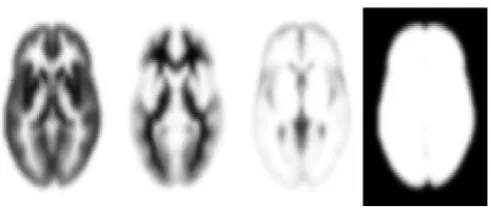
Figure 1: The a priori probability images of GM, WM, CSF and non-brain tissue. Values range between zero (white) and one (black).

voxel has been drawn. The intensities of voxels belonging to each of these clusters confirms to a normal distribution, which can be described by a mean, a variance and the number of voxels belonging to the distribution. For multi-spectral data (e.g. simultaneous segmentation of registered T2 and PD images), multivariate normal distributions can be used. In addition, the model has approximate knowledge of the spatial distributions of these clusters, in the form of prior probability images. Before using the current method for classifying an image, the image has to be in register with the prior probability images. The registration is normally achieved by least squares matching with template images in the same stereobatic space as the prior probability images. One of the greatest problems faced by tissue classification techniques is non-uniformity of the images intensity. Many groups have developed methods for correcting intensity non-uniformities, and the scheme developed here shares common features. There are two basic models describing image noise properties: multiplicative noise and additive noise.

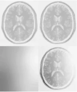
Figure . 2: The MR images are modelled as a number of distinct clusters (top left), with different levels of Gaussian random noise added to each cluster (top right). The intensity modulation is assumed to be smoothly varying (bottom left), and is applied as a straightforward multiplication of the modulation fieldwith the image (bottom right).

The current method uses a multiplicative noise model, which assumes that the errors originate from tissue variability rather

than additive Gaussian noise from the scanner. Figure. 2 illustrate the model used by the classification. Non-uniformity correction methods all involve estimating a smooth function that modulates the image intensities. The multiplicative model describes images that have noise added before being modulated by the non-uniformity eld (i.e., the standard deviation of the noise is multiplied by the modulating eld), whereas the additive version models noise that is added after the modulation (standard deviation is constant).

If the function is is not forced to be smooth, then it will begin to the higher frequency intensity variations due to different tissue types, rather than the low frequency intensity non-uniformity artefact. Spline [7, 4] and polynomial [5, 6] basis functions are widely used for modelling the intensity variation. In these models, the higher frequency intensity variations are restricted by limiting the number of basic functions. In the current method, a Bayesian model is used, where it is assumed that the modulation field (U) has been drawn from a population for which the a priori probability distribution is known, thus allowing high frequency variations of the modulation field to be penalized.

II. TISSUE CLASSIFICATION

The explanation of the tissue classification algorithm will be simplified by describing its application to a single two dimensional image. A number of assumptions are made by the classification model. The first is that each of the I x J voxels of the image (F) has been drawn from a known number (K) of distinct tissue classes (clusters). The distribution of the voxel intensities within each class is normal (or multi-normal for multi-spectral images) and initially unknown. The distribution of voxel intensities within cluster k is described by the number of voxels within the cluster (hk), the mean for that cluster (vk), and the variance around that mean (ck). Because the images are matched to a particular stereotaxic space, prior probabilities of the voxels belonging to the grey matter (GM), white matter (WM) and cerebra-spinal uid (CSF) classes are known. This information is in the form of probability images { provided by the Montreal Neurological Institute [9, 8, 10] as part of the ICBM, NIH P-20 project (Principal Investigator John Mazziotta), and derived from scans of 152 young healthy subjects. These probability images contain values in the range of zero to one, representing the prior probability of a voxel being either GM, WM or CSF after an image has been normalized to the same space (see Figure.1 ). The probability of a voxel at co-ordinate i; j belonging to cluster k is denoted by bijk.

assigned to each cluster requires the cluster parameters to be defined, and also the modulation field. In turn, estimating the modulation field needs the cluster parameters and the belonging probabilities.

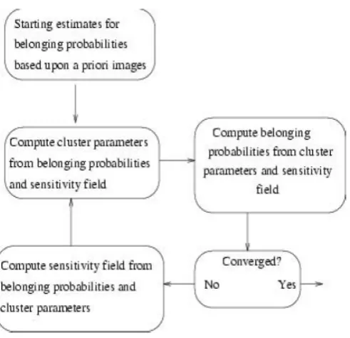
The problem requires an iterative algorithm (see Figure.3). It begins by assigning starting estimates for the various parameters. The starting estimate for the modulation field is typically uniformly one. Starting estimates for the belonging probabilities of the GM, WM and CSF partitions are based on the prior probability images. Since there are no prior probability maps for background and non-brain tissue clusters, they are estimated by subtracting the prior probabilities for GM, WM and CSF from a map of all ones, and dividing the result equally between the remaining clusters.

Figure .3: A flow diagram for the tissue classification.

Each iteration of the algorithm involves estimating the cluster parameters from the non-uniformity corrected image, assigning belonging probabilities based on the cluster parameters, checking for convergence, and re-estimating and applying the modulation function. With each iteration, the parameters describing the distributions move towards a better _t and the belonging probabilities (P) change slightly to reflect the new distributions. This continues until a convergence criterion is satisfied. The parameters describing clusters with corresponding prior probability images tend to converge more rapidly than the others. This may be partly due to the better starting estimates. The final values for the belonging probabilities are in the range of 0 to 1, although most values tend to stabilize very close to one of the two extremes. The algorithm is in fact an expectation maximization (EM) approach, where the E-step is the computation of the

belonging probabilities, and the M-step is the computation of the cluster and non-uniformity correction parameters. The individual steps involved in each iteration are now described in more detail.

1. Estimating the Cluster Parameters

This stage requires the most recent estimate of the modulation function (U, where uij is the multiplicative correction at voxel i; j), and the current estimate of the probability of voxel i; j belonging to class k, which is denoted by pijk. The first step is to compute the number of voxels (h) belonging to each of the K clusters as:

hk= Pijk over K=1….k

Mean voxel intensities for each cluster (v) are computed. This step effectively produces a weighted mean of the image voxels, where the weights are the current belonging probability estimates:

Uk= over K=1….k

Then the variance of each cluster (c) is computed in a similar way to the mean:

Ck =

2. Assigning Belonging Probabilities

The next step is to re-calculate the belonging probabilities. It uses the cluster parameters computed in the previous step, along with the prior probability images and the intensity modulated input image. Baye’s rule is used to assign the probability of each voxel belonging to each cluster:

Pijk= over i= 1....I, j=1...J, k=1...K

where pijk is the a posterior probability that voxel i; j belongs to cluster k given its intensity of fij , rijk is the likelihood of a voxel in cluster k having an intensity of fik, and sijk is the a priori probability of voxel i; j belonging in cluster k. The likelihood function is obtained by evaluating the probability density functions for the clusters at each of the voxels:

rijk= uij/(2 Ck)1/2 exp ( )

over i = 1::I, j = 1::J and k = 1::K.

probability images derived from a number of images (bijk). With no knowledge of the spatial prior probability distribution of the clusters or the intensity of a voxel, then the a priori probability of any voxel belonging to a particular cluster is proportional to the number of voxels currently included in that cluster. However, with the additional data from the prior probability images, a better estimate for the priors can be obtained:

Sijk=

over i = 1…..I, j = 1……J and k = 1…..K.

The algorithm is terminated when the change in log-likelihood from the previous iteration becomes negligible.

3 Estimating the Modulation Function

To reduce the number of parameters describing an intensity modulation field, it is modelled by a linear combination of low frequency discrete cosine transform (DCT) basis functions, which were chosen because there are no constraints at the boundary. A two (or three) dimensional discrete cosine transform (DCT) is performed as a series of one dimensional transforms, which are simply multiplications with the DCT matrix. The elements of a matrix (D) for computing the first M coefficients of the one dimensional DCT of a vector of length I is given by:

Di1= over i=1...I

Dim= over i=1...I, m=2..M

The matrix notation for computing the first Mx N coefficients of the two dimensional DCT of a modulation field U is Q = D1TUD2, where the dimensions of the DCT matrices D1 and D2 are IxM and JxN respectively, and U is an IxJ matrix. The

approximate inverse DCT is computed by U D1QD2 T . An alternative representation of the two dimensional DCT is obtained by reshaping the I x J matrix U so that it is a vector (u). Element i + (j - 1) x I of the vector is then equal to element i; j of the matrix. The two dimensional DCT can then be represented by q = DTu, where D = D2x D1 (the Kronecker tensor product of D2 and D1), and u ' Dq.

The sensitivity correction field is computed by re-estimating the coefficients (q) of the DCT basis functions such that the product of the likelihood and a prior probability of the parameters is increased. This can be formulated as an iteration of a Gauss-Newton optimisation algorithm.

q(n+1)= (C0-1+A) (C0-1 q0+A q(n)-b))

where q0 and C0 are the means and covariance matrices describing the a priori probability distribution of the coefficients. Vector b contains the first derivatives of the log-likelihood cost function with respect to the basis function

coefficients, and matrix A contains the second derivatives of the log-likelihood. These can be constructed efficiently using the properties of Kronecker tensor products.

III. CONCLUSIONS

The current segmentation method is fairly robust and accurate for high quality T1 weighted images, but is not beyond improvement. Currently, each voxel is assigned a probability of belonging to a particular tissue class based only on its intensity and information from the prior probability images. There is a great deal of other knowledge that could be incorporated into the classification. For example, if all a voxel's neighbours are grey matter, then there is a high probability that it should also be grey matter. Other researchers have successfully used Markov random field models to include this information in a tissue classification model [7, 12, 6, 13,14]. Another very simple prior, that can be incorporated, is the relative intensity of the different tissue types [10]. For example, when segmenting a T1 weighted image, it is known that the white matter should have a higher intensity than the grey matter, which in turn should be more intense than the CSF. When computing the means for each cluster, this prior information could sensibly be used to bias the estimates. In order to function properly, the classification method requires good contrast between the different tissue types. However, many central grey matter structures have image intensities that are almost indistinguishable from that of white matter, so the tissue classification is not always very accurate in these regions. Another related problem is that of partial volume. Because the model assumes that all voxels contain only one tissue type, the voxels that contain a mixture of tissues may not be modelled correctly. In particular, those voxels at the interface between white matter and ventricles will often appear as grey matter. Each voxel is assumed to be of only one tissue type, and not a combination of different tissues, so the model's assumptions are violated when voxels contain signal from more than one tissue type. This problem is greatest when the voxel dimensions are large, or if the images have been smoothed, and is illustrated using simulated data in Figure 4. The effect of partial volume is that it causes the distributions of the intensities to deviate from normal. Some authors have developed more complex models than mixtures of Gaussians to describe the intensity distributions of the classes [15]. A more recent commonly adopted approach involves modelling separate classes of partial volume voxels [13, 16, 17].

severely abnormal brains, as they are more difficult to register with images that represent the prior probabilities of voxels belonging to different classes. Segmenting such abnormal brains can be a problem for the algorithm, as the prior probability images are based on normal healthy brains. The profile in Figure 5 depends on the smoothness or resolution of the prior probability images. By not smoothing the prior probability images, the segmentation would be optimal for normal, young and healthy brains. However, these images may need to be smoother in order to encompass more variability when patient data are to be processed.

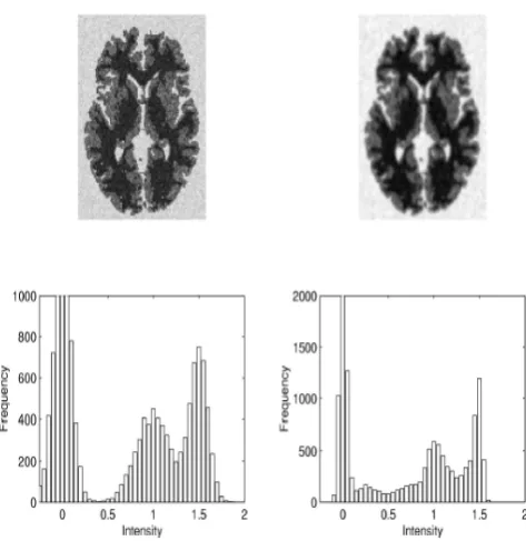
Figure 4: Simulated data showing the effects of partial volume on the intensity histograms. On the upper left is a simulated image consisting of three distinct clusters. The intensity histogram of this image is shown on the lower left and consists of three Gaussian distributions. The image at the top right is the simulated image after a small amount of smoothing. The corresponding intensity histogram no longer shows three distinct Gaussian distributions.

As an example, consider a subject with very large ventricles. CSF may appear where the priors suggest that tissue should always be WM. These CSF voxels are forced to be misclassified as WM, and the intensities of these voxels are incorporated into the computation of the WM means and variances. This results in the WM being characterized by a very broad distribution, so the algorithm is unable to distinguish it from any other tissue. For young healthy subjects, the classification is normally good, but caution is required when the method is used for severely pathological brains. MR images are normally reconstructed by taking the modulus of complex images. Normally distributed complex values are not normally distributed when the magnitude is taken. Instead, they obey a Rician distribution. This means

that any clusters representing the background are not well modelled by a single Gaussian, but it makes very little difference for most of the other clusters.

Figure 5: Segmentation accuracy with respect to misregistration with the prior probability images.

The segmentation is normally run on unprocessed brain images, where non-brain tissue is not first removed. This results in a small amount of non-brain tissue being classified as brain. However, by using morphological operations on the extracted GM and WM segments, it is possible to remove most of this extra tissue. The procedure begins by eroding the extracted WM image, so that any small specs of misclassified WM are removed. This is followed by conditionally dilating the eroded WM, such that dilation can only occur where GM and WM were present in the original extracted segments. Although some non-brain structures (such as part of the sagittal sinus) may remain after this processing, most non-brain tissue is removed.

REFERENCES

1. Linda G. Shapiro and George C. Stockman (2001): “Computer Vision”, pp 279-325, New Jersey, Prentice-Hall, ISBN 0-13-030796-3

2. J. A. Hartigan. Clustering Algorithms, pages 113{129. John Wiley & Sons, Inc., New York, 1975.

3. D.L. Collins, A.P. Zijdenbos, V. Kollokian, J.G. Sled, N.J. Kabani, C.J. Holmes and A.C. Evans. Design and construction of a realistic digital brain Phantom. IEEE Transactions on Medical Imaging, 17(3):463{468, 1998.

4. J. G. Sled, A. P. Zijdenbos, and A. C. Evans. A non-parametric method for automatic correction of intensity non-uniformity in MRI data. IEEE Transactions on Medical Imaging, 17(1):87{97, 1998.

6. K. Van Leemput, F. Maes, D. Vandermeulen, and P. Suetens. Automated model-based tissue classification of MR images of the brain. IEEE Transactions on Medical Imaging, 18(10):897{908, 1999.

7. M. X. H. Yan and J. S. Karp. An adaptive baysian approach to three- dimensional MR brain segmentation. In Y. Bizais, C. Barillot, and R. Di Paola, editors, Proc. Information Processing in Medical Imaging, pages 201{213, Dordrecht, The Netherlands, 1995. Kluwer Academic Publishers.

8. A. C. Evans, D. L. Collins, S. R. Mills, E. D. Brown, R. L. Kelly, and T. M. Peters. 3D statistical neuroanatomical models from 305 MRI volumes. In Proc. IEEE-Nuclear Science Symposium and Medical Imaging Conference, pages 1813{1817, 1993.

9. A. C. Evans, D. L. Collins, and B. Milner. An MRI-based stereotactic atlas from 250 young normal subjects. Society of Neuroscience Abstracts, 18:408, 1992.

10. A. C. Evans, M. Kamber, D. L. Collins, and D. Macdonald. An MRI- based probabilistic atlas of neuroanatomy. In S. Shorvon, D. Fish, F. Andermann, G. M. Bydder, and Stefan H, editors, Magnetic Resonance Scanning and Epilepsy, volume 264 of NATO ASI Series A, Life Sciences, pages 263{274. Plenum Press, 1994.

11. B. Fischl, D. H. Salat, E. Busa, M. Albert, M. Dieterich, C. Haselgrove, A. van der Kouwe, R. Killiany, D. Kennedy, S. Klaveness, A. Montillo, N. Makris, B. Rosen, and A. M. Dale. Whole brain segmentation: Automated labelling of neuroanatomical structures in the human brain. Neuron, 33:341{355, 2002.

12. D. Vandermeulen, X. Descombes, P. Suetens, and G. Marchal. Unsupervised regularized classification of multi-spectral MRI. In Proc. Visualization in Biomedical Computing, pages 229{234, 1996.

13 . S. Ruan, C. Jaggi, J. Xue, J. Fadili, and D. Bloyet. Brain tissue classification of magnetic resonance images using partial volume modelling. IEEE Transactions on Medical Imaging, 19(12):1179{1187, 2000.

14. Y. Zhang, M. Brady, and S. Smith. Segmentation of brain MR images through a hidden markov random field model and the expectation- maximization algorithm. IEEE Transactions on Medical Imaging, 20(1):45{57, 2001.

15. E. Bullmore, M. Brammer, G. Rouleau, B. Everitt, A. Simmons, T. Sharma, S. Frangou, R. Murray, and G. Dunn. Computerized brain tissue classification of magnetic resonance images: A new approach to the problem of partial volume artefact. NeuroImage, 2:133{147, 1995.

16. D. H. Laidlaw, K. W. Fleischer, and A. H. Barr. Partial-volume Bayesian classification of material mixtures in MR volume data using voxel histograms. IEEE Transactions on Medical Imaging, 17(1):74{86, 1998.