Available online: https://edupediapublications.org/journals/index.php/IJR/ P a g e | 545
Reweighted ZAQV- LMS Based Adaptive Beam Forming Array Sensor
STUDENT DETAILS:
Kanigolla Prem Manikanta Gupta
M.Tech(DECS), Department of ECE
Abstract— The aim of this paper is to provide efficient solution to
reduce the complexity of beamforming process and to reduce the energy consumption. In this letter an RZA-QLMS algorithm has been proposed for adaptive beamforming based on vector sensor arrays consisting of crossed dipoles. By using this technique in the process of beamforming the reduced system complexity and energy consumption can be achieved while an acceptable performance can still be maintained, which is especially useful for large array systems. Simulation results have shown that the proposed algorithm can work effectively for beamforming while enforcing a sparse solution for the weight vector where the corresponding crossed-dipole sensors with almost zero valued coefficients can be removed from the system.
Keywords:-vector sensor array, quaternion, adaptive beamforming, LMS, zero attracting.
I. INTRODUCTION
Adaptive beamforming has a range of applications and has been studied extensively in the past for traditional array systems [1], [2], [3], [4]. With the introduction of vector sensor arrays, such as those consisting of crossed-dipoles and tripoles [5], [6], [7], adaptive beamforming for such an array system has attracted more and more attention recently [6], [8], [9], [10].
In this work, we consider the crossed-dipole array and study the problem of how to reduce the number of sensors involved in the beamforming process so that reduced system complexity and energy consumption can be achieved while an acceptable performance can still be maintained, which is especially useful for large array systems. In particular, we will use the quaternion-valued steering vector model for crossed-
GUIDE DETAILS:
Suresh angadi
Assistant Professor
Department of ECE
dipole arrays [8], [9], [10], [11], [12], [13], [14], [15], [16], and propose a novel quaternion-valued adaptive algorithm for reference signal based beamforming.
In the past, several quaternion-valued adaptive filtering algo-rithms have been derived in [9], [16], [17], [18]. Notwithstand-ing the advantages of the quaternionic algorithms, extra cares have to be taken in their developments, in particular when the derivatives of quaternion-valued functions are involved, since
quaternion algebra is non-commutative. Very recently,
prop-erties and applications of a restricted HR1 gradient operator for quaternion-valued signal processing were provided in [19]. Based on these recent advances in quaternion-valued signal processing, we here derive a reweighted zero attracting (RZA) quaternion-valued least mean square (QLMS) algorithm by introducing a RZA term to the cost function of the QLMS algorithm. Similar to the idea of the RZA least mean square (RZA-LMS) algorithm proposed in [20], the RZA term aims
to have a closer approximation to the l0 norm so that the
number of non-zero valued coefficients can be reduced more effec-tively in the adaptive beamforming process. This algorithm can be considered as an extension of our recently proposed zero-attracting QLMS (ZA-QLMS) algorithm [21],
where the l1 norm penalty term was used in the update
equation of the weight vector. We will show in our
simulations that the RZA-LMS algorithm has a much better performance in terms of both steady state error and the number of sensors employed after convergence.
A review of adaptive beamforming based on vector sensor arrays is provided in Sec. II, and the proposed RZA-QLMS algorithm is derived in Sec. III. Simulations are presented in Sec. IV, and conclusions drawn in Sec. V.
II. ADAPTIVE BEAMFORMING BASED ON VECTOR
SENSOR ARRAYS
A. Quaternionic Array Signal Model
z
θ
...
φ d y
x
May 2017
Available online: https://edupediapublications.org/journals/index.php/IJR/ P a g e | 546
with a direction of arrival (DOA) defined by the angles θ and
d[
n
]+ e[
n
]ϕ, its spatial steering vector is given by
x1[
n
]− y [
n
]Sc(θ, ϕ) =
[1
, e
−j2πd sin θ sin ϕ/λ,
w1[n
]
. .
· · ·
, e−j2π(M−1)d sin θ sin ϕ/λ]T
(1)
. .
. .
where λ is the wavelength of the incident signal and {·}T xM[
n
] wM[n
]denotes the transpose operation. For a crossed dipole the
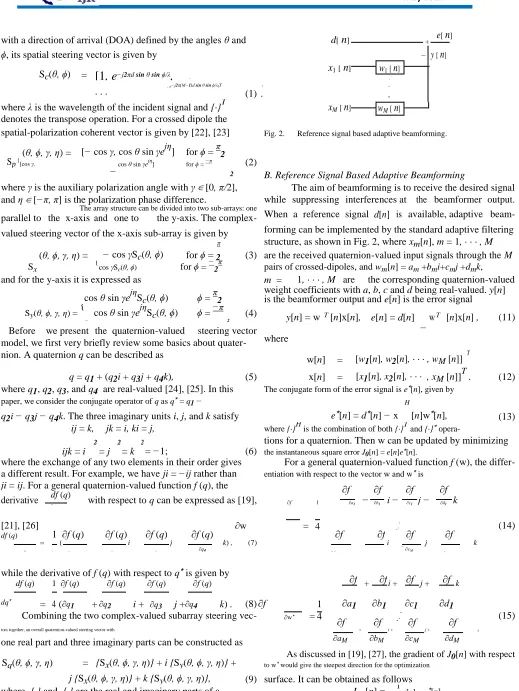
spatial-polarization coherent vector is given by [22], [23] Fig. 2. Reference signal based adaptive beamforming.
Sp
(θ, ϕ, γ, η) = [− cos γ, cos θ sin γejη] for ϕ = π2 (2) {
[cos γ,
− cos θ sin γe jη
] for ϕ = −π
2 B. Reference Signal Based Adaptive Beamforming
where γ is the auxiliary polarization angle with γ∈ [0, π/2], The aim of beamforming is to receive the desired signal
and η∈ [−π, π] is the polarization phase difference. while suppressing interferences at the beamformer output.
The array structure can be divided into two sub-arrays: one
When a reference signal d[n] is available, adaptive beam-
parallel to the x-axis and one to the y-axis. The complex-
forming can be implemented by the standard adaptive filtering valued steering vector of the x-axis sub-array is given by
structure, as shown in Fig. 2, where xm[n], m = 1,· · ·, M
− cos γSc(θ, ϕ)
π
(θ, ϕ, γ, η) =
for ϕ = 2 (3) are the received quaternion-valued input signals through the M
Sx {cos γSc(θ, ϕ) for ϕ = −
2
π
pairs of crossed-dipoles, and wm[n] = am +bmi+cmj +dmk,
and for the y-axis it is expressed as
m = 1,· · ·, M are
the corresponding quaternion-valued
cos θ sin γejηSc(θ, ϕ) ϕ =π2 weight coefficients with a, b, c and d being real-valued. y[n]
is the beamformer output and e[n] is the error signal
Sy(θ, ϕ, γ, η) =
{
cos θ sin γejηSc(θ, ϕ) ϕ =−π (4) y[n] =w T [n]x[n],
e[n] = d[n]
w T [n]x[n] , (11)
− 2
−
Before we present the quaternion-valued steering vector
where model, we first very briefly review some basics about quater-
nion. A quaternion q can be described as
w[n] = [w1[n], w2[n],· · ·, wM [n]] T
q = q1+ (q2i + q3j + q4k),
(5)
x[n]
=
[x1[n], x2[n],· · · , xM[n]]T . (12) where q1, q2, q3, and q4 are real-valued [24], [25]. In this The conjugate form of the error signal is e∗[n], given by
paper, we consider the conjugate operator of q as q∗ = q1−
e∗[n] = d∗[n] − x
H
[n]w∗[n],
(13)
q2i − q3j − q4k. The three imaginary units i, j, and k satisfy
ij = k, jk = i, ki = j, where {·}H is the combination of both {·}T and {·}∗ opera-
ijk = i
2
= j
2
= k
2
= −1;
(6)
tions for a quaternion. Then w can be updated by minimizing
the instantaneous square error J0[n] = e[n]e∗[n].
where the exchange of any two elements in their order gives For a general quaternion-valued function f (w), the differ-
a different result. For example, we have ji = −ij rather than entiation with respect to the vector w and w∗ is
ji = ij. For a general quaternion-valued function f (q), the ∂f ∂f ∂f ∂f df (q)
derivative with respect to q can be expressed as [19],
− i −
j − k
∂f 1 ∂a
1 ∂b1 ∂c1 ∂d1
dq
[21], [26] =
...
(14)
1 ∂f (q) ∂f (q) ∂f (q) ∂f (q) ∂w 4 ∂f ∂f ∂f ∂f
df (q)
= ( − i − j −
k) , (7) i j k
dq 4
∂q1 ∂q2 ∂q3 ∂aM − ∂bM
− ∂dM
∂q4
− ∂cM
while the derivative of f (q) with respect to q∗ is given by ∂f ∂f ∂f ∂f
df (q) 1 ∂f (q) ∂f (q) ∂f (q) ∂f (q) + i + j + k
(8) = ( +
i + j +
k) . ∂a1 ∂b1 ∂c1 ∂d1
dq∗ 4 ∂q
1 ∂q2 ∂q3 ∂q4 ∂f 1
Combining the two complex-valued subarray steering vec- ∂w∗ = 4 ... (15)
∂f ∂f ∂f ∂f
tors together, an overall quaternion-valued steering vector with + i + j + k
one real part and three imaginary parts can be constructed as ∂aM ∂bM ∂cM ∂dM
Sq(θ, ϕ, γ, η) = {Sx(θ, ϕ, γ, η)} + i {Sy(θ, ϕ, γ, η)} + to w∗ would give the steepest direction for the optimization As discussed in [19], [27], the gradient of J0[n] with respect
j {Sx(θ, ϕ, γ, η)} + k {Sy(θ, ϕ, γ, η)}, (9) surface. It can be obtained as follows
where {·} and {·} are the real and imaginary parts of a
∇w
J [n] =
− 1
e[n]
x
∗[n] ,
(16)
complex number/vector, respectively. Given a set of coeffi- 0
2
Available online: https://edupediapublications.org/journals/index.php/IJR/ P a g e | 547
r(θ, ϕ, γ, η) =w Sq(θ, ϕ, γ, η)
(10) µ is given by
w[n + 1] = w[n]
w J0[n],
(17)
where w is the quaternion-valued weight vector. µ
May 2017
Available online: https://edupediapublications.org/journals/index.php/IJR/ P a g e | 548
3
leading to the following QLMS algorithm [16], [17], [26]
w[n + 1] = w[n] + 1
µ(e[n]x∗[n]). (18)
2
III. THE RZA-QLMS ALGORITHM
Using the QLMS algorithm, we can find the optimal coef-ficient vector in terms of minimum mean square error (MSE) and obtain a satisfactory beamforming result. However, to reduce the complexity and also power consumption of the system, in particular for a large array, we can reduce the number of sensors involved, at the cost of the final beam-forming performance. To achieve this, we here derive a novel quaternion-valued adaptive algorithm by introducing an RZA term to the original cost function of the QLMS algorithm. In this way, we can simultaneously minimise the number of sensors involved while suppressing the interferences during the beamforming process.
First, to minimise the number of sensors, we could add the
l0norm of the weight vectorwto the cost function J0[n]to form a new cost function
J
ˆ
0[n] = (1 − δ1)e[n]e∗[n] + δ1∥w[n]∥0, (19)where δ1 is a weighting term between the original cost function and the newly introduced term. In this way, the number of non-zero valued coefficients in w will be minimised too, where the similar idea has been applied in [28].
In practice, we could replace the l0 norm by the l1 norm.
However, l1 norm would uniformly penalise all non-zero
valued coefficients, while l0 norm penalises smaller non-zero
values more heavily. To have a closer approximation to l0
norm, we can introduce a larger weighting term to those coefficients with smaller values and a smaller weighting term to those with larger values. This weighting term will change according to the resultant coefficients at each update of the algorithm. This general idea has been implemented as a
reweighted l1 minimization [29], [30] and employed in the
sparse array design problem [31], [32], [33].
The modified cost function for the proposed RZA-QLMS algorithm with the reweighting term is given by
∑
MJ1[n] = (1 − δ1)e[n]e∗[n] + δ1 (εm|wm[n]|), (20)
m=1
where εm is the reweighting term for wm. Then using the chain
rule in [19], we can obtain the gradient of J1[n] with respect to
w∗[n]. In particular, the differentiation of the second part of
J1[n] with regards to wm∗[n] is given by
∂(εm|wm[n]|)
TABLE I
COMPARISON OF COMPUTATIONAL COMPLEXITY.
QLMS ZA-QLMS RZA-QLMS
Real-valued addition 28M+4 35M+4 38M+4
Real-valued multiplication 32M+4 44M+4 52M+4
(Including square root operation) (0) (M) (2M)
where sign(·) is a component-wise sign function
sign(w
[n]) = wm[n]/|wm[n]| wm[n] = 0
m
{
0
wm[n] = 0
The overall gradient result is given by
w J [n] =
1 (1 δ )e[n]x
∗ [n] + 1 δ ε (sign(w [n])).
m m
∇ 1
−2 −
1 m
4
1
m (22)
We choose the reweighting term εm as
εm= 1/(ζ + |wm[n]|),
(23)
with ζ being roughly the threshold value below which the
corresponding sensor will not be included in the update. Then, with the step size µ1, we finally obtain the following update equation for the RZA-QLMS algorithm in vector form
w[n + 1] = w[n] +
1
(µ1 − 4ρ1)(e[n]x∗[n]) 2
−ρ1(sign(w[n]))./(ζ + |w[n]|) , (24)
where ρ1 = 14µ1δ1, |w[n]| is a vector formed by taking the
absolute value of the coefficients in w[n], „./‟ is a
component-wise division between two vectors, and sign(w[n]) is defined as {
w[n]./|w[n]| w[n] = 0
sign(w[n]) =
0 w[n] = 0
When ζ + |w[n]| is removed from the above equation, it will
be reduced to the ZA-QLMS algorithm in [21], with its cost function given by
J2[n] = (1 − δ2)e[n]e∗[n] + δ2∥w[n]∥1 , (25)
where δ2 is a trade-off factor. The update equation for the
ZA-QLMS algorithm is
w[n + 1] = w[n] +
1
2
(µ2− 4ρ2)(e[n]x∗[n]) −ρ2·sign(w[n]) ,(26) where ρ2 = 14µ2δ2, and µ2 is the step size.
We now discuss the computational complexity of the
al-gorithms. The results are shown in Tab. I, where M is the
number of vector sensors of the array. Obviously, the RZA-QLMS algorithm has the highest complexity. However, as we will see in simulations, this additional cost is paid back by a
∂wm∗ = 1εm(∂(|wm
[n]|) +∂(|wm
[n]|)
i
4∂am∂bm
+ ∂(|wm[n]|) j + ∂(|wm[n]|) k)
∂cm ∂dm
1 am bm cm
= εm( + i +
j +
4 |wm[n]| |wm[n]| |wm[n]|
=
1
εm
w
m
[
n
]
=
1
Available online: https://edupediapublications.org/journals/index.php/IJR/ P a g e | 549 dm |wm[n]|
k
)
(21) much smaller number of sensors, and especially at a later stage of the adaptation,
when the
number of sensors involved becomes smaller, the overall complexity of the RZA-QLMS algorithm
could be
lower than
the other
two algorithms.
After removing the sensors
with a
smaller magnitude
for their
coefficients compared
to ζ, the
beam response difference ∆r between the original
array and
the new
one is
given by
∆r = |wHSq − (w − ∆w)HSq|
√
May 2017
Available online: https://edupediapublications.org/journals/index.php/IJR/ P a g e | 550
0
QLMS
ZA−QLMS
[d
B
]
−5 RZA−QLMS
E
rr
o
r
M
e
a
n
S
q
u
a
re −10
−15
N o r m a l i s e d
−20
E
n
s
e
m
b
le
−25
−30
1000 2000 3000 4000 5000 6000 7000 8000 0
Iterations
where ∆M is the number of removed sensors, and ∆w is the
change of w after some of its sensors are removed (the corresponding coefficients on the positions of removed sensors
have a magnitude smaller than ζ and are then set to zero). As
a result, the maximum possible change in array response, due
√
to removal of some sensors, is given by ζ· ∆M· M .
IV. SIMULATION RESULTS
Using the QLMS algorithm, we can find the optimal coefficient vector and obtain a satisfactory beamforming result as shown in below figure. However, to reduce the complexity and also power consumption of the system, in particular for a large array, at the cost of the final beamforming performance. To achieve this, we here derive a novel quaternion-valued adaptive algorithm by introducing an RZA term to the original cost function of the QLMS algorithm. In this way, we can simultaneously minimise the number of sensors involved while suppressing the interferences during the beamforming process.
Comparision of MSE
we see that although these three algorithms have a similar convergence speed, the original QLMS algorithm has the smallest steady state error, which is not surprising since it has
the most degrees of freedom among them. On the other hand, the proposed RZA-QLMS algorithm has achieved a lower steady state error than the ZA-QLMS algorithm.
Spectral Density
Beampattern of all three algorithms are drawn in above results. From the above simulation results we have observed RZA QLMS have satisfactory beamforming results.
Available online: https://edupediapublications.org/journals/index.php/IJR/ P a g e | 551 Beam pattern of proposed RZA-QLMS algorithm has been
shown in above figure. It can reduce system complexity and energy consumption can be achieved while an acceptable performance can still be maintained, which is especially useful for large array systems. Simulation results have shown that the proposed algorithm can work effectively for beamforming while enforcing a sparse solution for the weight
almost zero valued coefficients can be removed from the system.
V. CONCLUSION
An RZA-QLMS algorithm has been proposed for adaptive beamforming based on vector sensor arrays consisting of crossed dipoles. It can reduce the number of sensors involved in the beamforming process so that reduced system complexity and energy consumption can be achieved while an acceptable performance can still be maintained, which is especially useful for large array systems. Simulation results have shown that the proposed algorithm can work effectively for beamforming while enforcing a sparse solution for the weight vector where the corresponding crossed-dipole sensors with almost zero-valued coefficients can be removed from the system.
REFERENCES
[1] H. L. Van Trees, Optimum Array Processing, Part IV of Detection,
Estimation, and Modulation Theory. New York: Wiley, 2002.
[2] W. Liu and S. Weiss, Wideband Beamforming: Concepts and
Techniques. Chichester, UK: John Wiley & Sons, 2010.
[3] C. G. Li, F. Sun, J. M. Cioffi, and L. X. Yang, “Energy Efficient MIMO
Relay Transmissions via Joint Power Allocations ,” IEEE Transactions
on Circuits & Systems II: Express Briefs, vol. 61, no. 7, pp. 531–535, July 2014.
[4] X. C. Chen, W. Zhang, W. Rhee, and Z. H. Wang, “A ∆Σ TDC-based
beamforming method for vital sign detection radar systems,” IEEE
Transactions on Circuits & Systems II: Express Briefs, vol. 61, no. 12,
pp. 932–936, December 2014.
[5] R. T. Compton, “The tripole antenna: An adaptive array with full
po-larization flexibility,” IEEE Transactions on Antennas and Propagation,
vol. 29, no. 6, pp. 944–952, November 1981.
[6] A. Nehorai, K. C. Ho, and B. T. G. Tan, “Minimum-noise-variance
beamformer with an electromagnetic vector sensor,” IEEE Transactions
on Signal Processing, vol. 47, no. 3, pp. 601–618, March 1999.
[7] M. D. Zoltowski and K. T. Wong, “ESPRIT-based 2D direction finding
with a sparse uniform array of electromagnetic vector-sensors,” IEEE
Transactions on Signal Processing, vol. 48, no. 8, pp. 2195–2204,
August 2000.
[8] X. M. Gou, Y. G. Xu, Z. W. Liu, and X. F. Gong, “Quaternion-Capon
beamformer using crossed-dipole arrays,” in Proc. IEEE International
Symposium on Microwave, Antenna, Propagation, and EMC
Technolo-gies for Wireless Communications (MAPE), November 2011, pp. 34–37.
[9] X. R. Zhang, W. Liu, Y. G. Xu, and Z. W. Liu, “Quaternion-valued
robust adaptive beamformer for electromagnetic vector-sensor arrays
with worst-case constraint,” Signal Processing, vol. 104, pp. 274–283,
November 2014.
[10] M. B. Hawes, and W. Liu, “Design of fixed beamformers based on
vector-sensor arrays,” International Journal of Antennas and
Propaga-tion, vol. 2015, 2015.
[11] N. Le Bihan and J. Mars, “Singular value decomposition of quaternion
matrices: a new tool for vector-sensor signal processing,” Signal
Pro-cessing, vol. 84, no. 7, pp. 1177–1199, 2004.
[12] S. Miron, N. Le Bihan, and J. I. Mars, “Quaternion-MUSIC for
vector-sensor array processing,” IEEE Transactions on Signal Processing, vol.
54, no. 4, pp. 1218–1229, April 2006.
[13] N. Le Bihan, S. Miron, and J. I. Mars, “MUSIC algorithm for
vector-sensors array using biquaternions,” IEEE Transactions on Signal
Pro-cessing, vol. 55, no. 9, pp. 4523–4533, 2007.
[14] J. W. Tao and W. X. Chang, “A novel combined beamformer based on
hypercomplex processes,” IEEE Transactions on Aerospace and
Electronic Systems, vol. 49, no. 2, pp. 1276–1289, 2013.
[15] J. W. Tao, “Performance analysis for interference and noise canceller
based on hypercomplex and spatio-temporal-polarisation processes,”
IETRadar, Sonar Navigation, vol. 7, no. 3, pp. 277–286, 2013.
[16] J. W. Tao and W. X. Chang, “Adaptive beamforming based on complex
quaternion processes,” Mathematical Problems in Engineering, vol.
2014, 2014.
[17] Q. Barthelemy,´ A. Larue, and J. I. Mars, “About QLMS derivations,”
IEEE Signal Processing Letters, vol. 21, no. 2, pp. 240–243, 2014.
[18] W. Liu, “Channel equalization and beamforming for quaternion-valued
wireless communication systems,” Journal of the Franklin Institute
(arXiv:1506.00231 [cs.IT]), November 2015.
[19] M. D. Jiang, Y. Li, and W. Liu, “Properties and applications of a
restricted HR gradient operator,” arXiv:1407.5178 [math.OC], July
2014.
[20] Y. Chen, Y. Gu, and A. O. Hero, “Sparse LMS for system
identification,” in Proc. IEEE International Conference on Acoustics,
Speech, andSignal Processing, Taipei, April 2009, pp. 3125–3128.
[21] M. D. Jiang, W. Liu, and Y. Li, “A zero-attracting quaternion-valued
least mean square algorithm for sparse system identification,” in Proc.
of IEEE/IET International Symposium on Communication Systems,
Net-works and Digital Signal Processing, Manchester, UK, July 2014.
[22] R. Compton, “On the performance of a polarization sensitive adaptive
array,” IEEE Transactions on Antennas and Propagation, vol. 29, no. 5,
pp.718–725, 1981.
[23] J. Li and R. Compton Jr, “Angle and polarization estimation using esprit
with a polarization sensitive array,” IEEE Transactions on Antennas and
Propagation, vol. 39, pp. 1376–1383, 1991.
[24] W. R. Hamilton, Elements of quaternions. Longmans, Green, & co.,
1866.
[25] I. Kantor, A. Solodovnikov, and A. Shenitzer, Hypercomplex numbers:
an elementary introduction to algebras. New York: Springer Verlag,
1989.
[26] M. D. Jiang, W. Liu, and Y. Li, “A general quaternion-valued gradient
operator and its applications to computational fluid dynamics and
adaptive beamforming,” in Proc. of the International Conference on
Digital Signal Processing, Hong Kong, August 2014.
[27] D. H. Brandwood, “A complex gradient operator and its application in
adaptive array theory,” IEE Proceedings H (Microwaves, Optics and
Antennas), vol. 130, no. 1, pp. 11–16, 1983.
[28] J. Yoo, J. Shin, and P. Park, “An improved NLMS algorithm in sparse
systems against noisy input signals,” IEEE Transactions on Circuits &
Systems II: Express Briefs, vol. 62, no. 3, pp. 271–275, March 2015.
[29] E. J. Cand`es, M. B. Wakin, and S. P. Boyd, “Enhancing sparsity by
reweighted l1 minimization,” Journal of Fourier Analysis and
Applica-tions, vol. 14, pp. 877–905, 2008.
[30] W. Xu, J. X. Zhao, and C. Gu, “Design of linear-phase FIR
multiple-notch filters via an iterative reweighted OMP scheme,” IEEE
Trans-actions on Circuits & Systems II: Express Briefs, vol. 61, no. 10, pp. 813–817, October 2014.
[31] B. Fuchs, “Synthesis of sparse arrays with focused or shaped
beam-pattern via sequential convex optimizations,” IEEE Transactions on
Antennas and Propagation, vol. 60, no. 7, pp. 3499–3503, 2012.
[32] G. Prisco and M. D‟Urso, “Maximally sparse arrays via sequential
con-vex optimizations,” IEEE Antennas and Wireless Propagation Letters,
vol. 11, pp. 192–195, 2012.
[33] M. B. Hawes, and W. Liu, “Compressive sensing based approach to the
design of linear robust sparse antenna arrays with physical size
constraint”, IET Microwaves, Antennas & Propagation, vol. 8, issue 10,