An Interactive Spreadsheet for Teaching the Forward-Backward Algorithm
Jason Eisner
Department of Computer Science Johns Hopkins University Baltimore, MD, USA 21218-2691
Abstract
This paper offers a detailed lesson plan on the forward-backward algorithm. The lesson is taught from a live, com-mented spreadsheet that implements the algorithm and graphs its behavior on a whimsical toy example. By experimenting with different inputs, one can help students develop intuitions about HMMs in particular and Expectation Maximization in general. The spreadsheet and a coordinated follow-up assign-ment are available.
1 Why Teach from a Spreadsheet?
Algorithm animations are a wonderful teaching tool. They are concrete, visual, playful, sometimes inter-active, and remain available to students after the lec-ture ends. Unfortunately, they have mainly been lim-ited to algorithms that manipulate easy-to-draw data structures.
Numerical algorithms can be “animated” by
spreadsheets. Although current spreadsheets do not provide video, they can show “all at once” how a computation unfolds over time, displaying interme-diate results in successive rows of a table and on graphs. Like the best algorithm animations, they let the user manipulate the input data to see what changes. The user can instantly and graphically see the effect on the whole course of the computation.
Spreadsheets are also transparent. In Figure 1, the user has double-clicked on a cell to reveal its un-derlying formula. The other cells that it depends on are automatically highlighted, with colors keyed to the references in the formula. There is no program-ming language to learn: spreadsheet programs are aimed at the mass market, with an intuitive design and plenty of online help, and today’s undergrad-uates already understand their basic operation. An adventurous student can even experiment with mod-ifying the formulas, or can instrument the spread-sheet with additional graphs.
[image:1.612.315.532.179.230.2]Finally, modern spreadsheet programs such as Microsoft Excel support visually attractive layouts with integrated comments, color, fonts, shading, and
Figure 1: User has double-clicked on cell D29.
drawings. This makes them effective for both class-room presentation and individual study.
This paper describes a lesson plan that was cen-tered around a live spreadsheet, as well as a subse-quent programming assignment in which the spread-sheet served as a debugging aid. The materials are available for use by others.
Students were especially engaged in class, appar-ently for the following reasons:
• Striking results (“It learned it!”) that could be im-mediately apprehended from the graphs.
• Live interactive demo. The students were eager to guess what the algorithm would do on partic-ular inputs and test their guesses.
• A whimsical toy example.
• The departure from the usual class routine. • Novel use of spreadsheets. Several students who
thought of them as mere bookkeeping tools were awed by this, with one calling it “the coolest-ass spreadsheet ever.”
2 How to Teach from a Spreadsheet?
It is possible to teach from a live spreadsheet by us-ing an RGB projector. The spreadsheet’s zoom fea-ture can compensate for small type, although under-graduate eyes prove sharp enough that it may be un-necessary. (Invite the students to sit near the front.)
Of course, interesting spreadsheets are much too big to fit on the screen, even with a “View / Full Screen” command. But scrolling is easy to follow if it is not too fast and if the class has previously
been given a tour of the overall spreadsheet layout (by scrolling and/or zooming out). Split-screen fea-tures such as hide rows/columns, split panes, and freeze panes can be moderately helpful; so can com-mands to jump around the spreadsheet, or switch be-tween two windows that display different areas. It is a good idea to memorize key sequences for such
commands rather than struggle with mouse menus
or dialog boxes during class.
3 The Subject Matter
Among topics in natural language processing, the forward-backward or Baum-Welch algorithm (Baum, 1972) is particularly difficult to teach. The algorithm estimates the parameters of a Hidden Markov Model (HMM) by Expectation-Maximization (EM), using dynamic programming to carry out the expectation steps efficiently.
HMMs have long been central in speech recog-nition (Rabiner, 1989). Their application to part-of-speech tagging (Church, 1988; DeRose, 1988) kicked off the era of statistical NLP, and they have found additional NLP applications to phrase chunk-ing, text segmentation, word-sense disambiguation, and information extraction.
The algorithm is also important to teach for ped-agogical reasons, as the entry point to a family of EM algorithms for unsupervised parameter estima-tion. Indeed, it is an instructive special case of (1) the inside-outside algorithm for estimation of prob-abilistic context-free grammars; (2) belief propa-gation for training singly-connected Bayesian net-works and junction trees (Pearl, 1988; Lauritzen, 1995); (3) algorithms for learning alignment mod-els such as weighted edit distance; (4) general finite-state parameter estimation (Eisner, 2002).
Before studying the algorithm, students should first have worked with some if not all of the key ideas in simpler settings. Markov models can be introduced through n-gram models or probabilistic finite-state automata. EM can be introduced through simpler tasks such as soft clustering. Global opti-mization through dynamic programming can be in-troduced in other contexts such as probabilistic CKY parsing or edit distance. Finally, the students should understand supervised training and Viterbi decod-ing of HMMs, for example in the context of
part-of-speech tagging.
Even with such preparation, however, the forward-backward algorithm can be difficult for be-ginning students to apprehend. It requires them to think about all of the above ideas at once, in com-bination, and to relate them to the nitty-gritty of the algorithm, namely
• the two-pass computation of mysteriousαandβ
probabilities
• the conversion of these prior path probabilities to posterior expectations of transition and emission counts
Just as important, students must develop an under-standing of the algorithm’s qualitative properties, which it shares with other EM algorithms:
• performs unsupervised learning (what is this and why is it possible?)
• alternates expectation and maximization steps • maximizes p(observed training data) (i.e., total
probability of all hidden paths that generate those data)
• finds only a local maximum, so is sensitive to initial conditions
• cannot escape zeroes or symmetries, so they should be avoided in initial conditions
• uses the states as it sees fit, ignoring the sugges-tive names that we may give them (e.g., part of speech tags)
• may overfit the training data unless smoothing is used
The spreadsheet lesson was deployed in two 50-minute lectures at Johns Hopkins University, in an introductory NLP course aimed at upper-level un-dergraduates and first-year graduate students. A sin-gle lecture might have sufficed for a less interactive presentation.
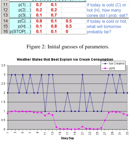
Figure 2: Initial guesses of parameters.
Figure 3: Diary data and reconstructed weather.
4 The Ice Cream Climatology Data
[While the spreadsheet could be used in many ways, the next several sections offer one detailed lesson plan. Questions for the class are included; subse-quent points often depend on the answers, which are concealed here in footnotes. Some fragments of the full spreadsheet are shown in the figures.]
The situation: You are climatologists in the year 2799, studying the history of global warming. You can’t find any records of Baltimore weather, but you do find my diary, in which I assiduously recorded how much ice cream I ate each day (see Figure 3).
What can you figure out from this about the weather that summer?
Let’s simplify and suppose there are only two kinds of days: C(cold) andH(hot). And let’s sup-pose you have guessed some probabilities as shown on the spreadsheet (Figure 2).
Thus, you guess that on cold days, I usually ate only 1 ice cream cone: my probabilities of 1, 2, or 3 cones were 70%, 20% and 10%. That adds up to 100%. On hot days, the probabilities were reversed—I usually ate 3 ice creams. So other things equal, if you know I ate 3 ice creams, the odds are 7 to 1 that it was a hot day, but if I ate 2 ice creams,
the odds are 1 to 1 (no information).
You also guess (still Figure 2) that if today is cold, tomorrow is probably cold, and if today is hot, to-morrow is probably hot. (Q: How does this setup resemble part-of-speech tagging?1)
We also have some boundary conditions. I only kept this diary for a while. If I was more likely to start or stop the diary on a hot day, then that is use-ful information and it should go in the table. (Q: Is there an analogy in part-of-speech tagging?2) For simplicity, let’s guess that I was equally likely to start or stop on a hot or cold day. So the first day I started writing was equally likely (50%) to be hot or cold, and any given day had the same chance (10%) of being the last recorded day, e.g., because on any day I wrote (regardless of temperature), I had a 10% chance of losing my diary.
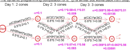
5 The Trellis andαβ Decoding
[The notationpi(H)in this paper stands for the
prob-ability ofHon dayi, given all the observed ice cream data. On the spreadsheet itself the subscript i is clear from context and is dropped; thus in Figure 3,
p(H)denotes the conditional probabilitypi(H), not a
prior. The spreadsheet likewise omits subscripts on
αi(H)andβi(H).]
Scroll down the spreadsheet and look at the lower line of Figure 3, which shows a weather reconstruc-tion under the above assumpreconstruc-tions. It estimates the relative hot and cold probabilities for each day. Ap-parently, the summer was mostly hot with a cold spell in the middle; we are unsure about the weather on a few transitional days.
We will now see how the reconstruction was ac-complished. Look at the trellis diagram on the spreadsheet (Figure 4). Consistent with visual intu-ition, arcs (lines) represent days and states (points) represent the intervening midnights. A cold day is represented by an arc that ends in a C state.3 (So
1
A: This is a bigram tag generation model with tagsCandH. Each tag independently generates a word (1, 2, or 3); the word choice is conditioned on the tag.
2
A: A tagger should know that sentences tend to start with
determiners and end with periods. A tagging that ends with a determiner should be penalized becausep(Stop|Det)≈0.
3
[image:3.612.71.289.88.328.2]Figure 4: Theα-βtrellis.
each arc effectively inherits the C orH label of its terminal state.)
Q: According to the trellis, what is the a priori probability that the first three days of summer are
H,H,Cand I eat 2,3,3 cones respectively (as I did)?4 Q: Of the 8 ways to account for the 2,3,3 cones, which is most probable?5 Q: Why do all 8 paths have low probabilities?6
Recall that the Viterbi algorithm computes, at each state of the trellis, the maximum probability of any path from Start. Similarly, define α at a state to be the total probability of all paths to that state fromStart. Q: How would you compute it by dynamic programming?7Q: Symmetrically, how would you computeβat a state, which is defined to be the total probability of all paths toStop?
The αandβvalues are computed on the spread-sheet (Figure 1). Q: Are there any patterns in the values?8
Now for some important questions. Q: What is the total probability of all paths from Start to
would bear emission probabilities such asp(3|H). In Figure 4, as in finite-state machines, this role is played by the arcs (which also carry transition probabilities such asp(H|C)); this allows
αandβto be described more simply as sums of path probabili-ties. But we persist in a traditional labeling of the states asHor
Cso that theαβnotation can refer to them.
4A: Consult the pathStart →H → H→ C, which has
probability(0.5·0.2)·(0.8·0.7)·(0.1·0.1) = 0.1·0.56·0.01 = 0.00056. Note that the trellis is specialized to these data.
5
A: H,H,H gives probability0.1·0.56·0.56 = 0.03136. (Starting withCwould be as cheap as starting withH, but then getting fromCtoHwould be expensive.)
6
A: It was a priori unlikely that I’d eat exactly this sequence
of ice creams. (A priori there were many more than 8 possible paths, but this trellis only shows the paths generating the actual data 2,3,3.) We’ll be interested in the relative probabilities of these 8 paths.
7
A: In terms of αat the predecessor states: just replace “max” with “+” in the Viterbi algorithm.
8
A:αprobabilities decrease going down the column, andβ
[image:4.612.75.286.76.158.2]probabilities decrease going up, as they become responsible for generating more and more ice cream data.
Figure 5: Computing expected counts and their totals.
Stop in which day 3 is hot?9 It is shown in col-umn H of Figure 1. Q: Why is colcol-umn I of Figure 1 constant at 9.13e-19 across rows?10 Q: What does that column tell us about ice cream or weather?11
Now the class may be able to see how to complete the reconstruction:
p(day 3 hot|2,3,3, . . .) = p(day 3 hot,2,3,3,...)p(2,3,3,...)
= α3(H)·β3(H)
α3(C)·β3(C)+α3(H)·β3(H) =
9.0e-19 9.8e-21+9.0e-19
which is 0.989, as shown in cell K29 of Figure 5. Figure 3 simply graphs column K.
6 Understanding the Reconstruction
Notice that the lower line in Figure 3 has the same general shape as the upper line (the original data), but is smoother. For example, some 2-ice-cream days were tagged as probably cold and some as probably hot. Q: Why?12 Q: Since the first day has 2 ice creams and doesn’t follow a hot day, why was it tagged as hot?13 Q: Why was day 11, which has only 1 ice cream, tagged as hot?14
We can experiment with the spreadsheet (using the Undo command after each experiment). Q: What do you predict will happen to Figure 3 if we weaken
9
A: By the distributive law,α3(H)·β3(H).
10A: It is the total probability of all paths that go through
ei-therCorHon a given day. But all paths do that, so this is simply the total probability of all paths! The choice of day doesn’t mat-ter.
11
A: It is the probability of my actual ice cream consumption: p(2,3,3, . . .) = P
~
wp(w,~ 2,3,3, . . .) =9.13e-19, wherew~
ranges over all233 possible weather state sequences such as
H,H,C,. . . . Each summand is the probability of a trellis path.
12
A: Figure 2 assumed a kind of “weather inertia” in which
a hot day tends to be followed by another hot day, and likewise for cold days.
13
Because an apparently hot day follows it. (See footnote 5.) It is theβfactors that consider this information from the future, and makeα1(H)·β1(H)α1(C)·β1(C).
14
A: Switching from hot to cold and back (HCH) has proba-bility 0.01, whereas staying hot (HHH) has probability 0.64. So although the fact that I ate only one ice cream on day 11 favors
Cby 7 to 1, the inferred “fact” that days 10 and 12 are hot favors
(a)
[image:5.612.72.300.65.369.2](b)
Figure 6: With (a) no inertia, and (b) anti-inertia.
or remove the “weather inertia” in Figure 2?15 Q: What happens if we try “anti-inertia”?16
Even though the number of ice creams is not de-cisive (consider day 11), it is influential. Q: What do you predict will happen if the distribution of ice creams is the same on hot and cold days?17 Q: What if we also changep(H|Start)from 0.5 to 0?18
7 Reestimating Emission Probabilities
We originally assumed (Figure 2) that I had a 20% chance of eating 2 cones on either a hot or a cold day. But if our reconstruction is right (Figure 3), I
actually ate 2 cones on 20% of cold days but 40+%
of hot days.
15A: Changingp(C| C) =p(H |C) =p(C |H) =p(H| H) = 0.45cancels the smoothing effect (Figure 6a). The lower line now tracks the upper line exactly.
16A: Settingp(C
| H) =p(H |C) = 0.8andp(C| C) =
p(H|H) = 0.1, rather than vice-versa, yields Figure 6b.
17
A: The ice cream data now gives us no information about
the weather, sopi(H) =pi(C) = 0.5on every dayi.
18
A: p1(H) = 0, butpi(H)increases toward an asymptote of 0.5 (the “limit distribution”). The weather is more likely to
switch to hot than to cold if it was more likely cold to begin
[image:5.612.315.531.71.170.2]with; sopi(H)increases if it is<0.5.
Figure 7: Parameters of Figure 2 updated by reestimation.
So now that we “know” which days are hot and which days are cold, we should really update our probabilities to 0.2 and 0.4, not 0.2 and 0.2. After all, our initial probabilities were just guesses.
Q: Where does the learning come from—isn’t this circular? Since our reconstruction was based on the guessed probabilities 0.2 and 0.2, why didn’t the re-construction perfectly reflect those guesses?19
Scrolling rightward on the spreadsheet, we find a table giving the updated probabilities (Figure 7). This table feeds into a second copy of the forward-backward calculation and graph. Q: The second graph ofpi(H) (not shown here) closely resembles
the first; why is it different on days 11 and 27?20 The updated probability table was computed by the spreadsheet. Q: When it calculated how often I ate 2 cones on a reconstructed hot day, do you think it counted day 27 as a hot day or a cold day?21
8 Reestimating Transition Probabilities
Notice that Figure 7 also updated the transition prob-abilities. This involved counting the 4 kinds of days distinguished by Figure 8:22 e.g., what fraction ofH
19
A: The reconstruction of the weather underlying the
ob-served data was a compromise between the guessed probabili-ties (Figure 2) and the demands of the actual data. The model in Figure 2 disagreed with the data: it would not have predicted that 2-cone days actually accounted for more than 20% of all days, or that they were disproportionately likely to fall between 3-cone days.
20
A: These days fall between hot and cold days, so smoothing
has little effect: their temperature is mainly reconstructed from the number of ice creams. 1 ice cream is now better evidence of a cold day, and 2 ice creams of a hot day. Interestingly, days 11 and 14 can now conspire to “cool down” the intervening 3-ice-cream days.
21
A: Half of each, sincep27(H) ≈0.5! The actual compu-tation is performed in Figure 5 and should be discussed at this point.
22
Figure 8: Second-order weather reconstruction.
days were followed byH? Again, fractional counts were used to handle uncertainty.
Q: Does Figure 3 (first-order reconstruction) contain enough information to construct Figure 8 (second-order reconstruction)?23
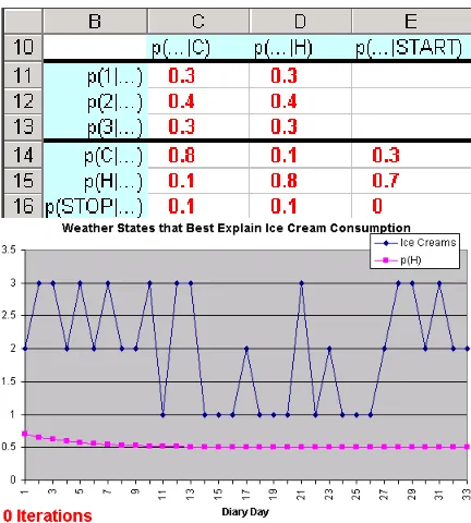
Continuing with the probabilities from the end of footnote 23, suppose we increasep(H | Start)to 0.7. Q: What will happen to the first-order graph?24 Q: What if we switch from anti-inertia back to iner-tia (Figure 9)?25
Q: In this last case, what do you predict will hap-pen when we reestimate the probabilities?26
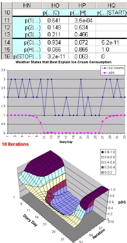
This reestimation (Figure 10) slightly improved the reconstruction. [Defer discussion of what “im-proved” means: the class still assumes that good re-constructions look like Figure 3.] Q: Now what? A: Perhaps we should do it again. And again, and again. . . Scrolling rightward past 10 successive rees-timations, we see that this arrives at the intuitively
23
A: No. A dramatic way to see this is to make the
dis-tribution of ice cream disdis-tribution the same on hot and cold days. This makes the first-order graph constant at 0.5 as in foot-note 17. But we can still get a range of behaviors in the second-order graph; e.g., if we switch from inertia to anti-inertia as in footnote 16, then we switch from thinking the weather is un-known but constant to thinking it is unun-known but oscillating.
24
A:pi(H)alternates and converges to 0.5 from both sides.
25
A:pi(H)converges to 0.5 from above (cf. footnote 18), as shown in Figure 9.
26A: The first-order graph suggests that the early days of
[image:6.612.74.288.73.227.2]summer were slightly more likely to be hot than cold. Since we ate more ice cream on those days, the reestimated probabili-ties (unlike the initial ones) slightly favor eating more ice cream on hot days. So the new reconstruction based on these proba-bilities has a very shallow “U” shape (bottom of Figure 10), in which the low-ice-cream middle of the summer is slightly less likely to be hot.
Figure 9: An initial poor reconstruction that will be improved by reestimation.
correct answer (Figure 11)!
Thus, starting from an uninformed probability ta-ble, the spreadsheet learned sensible probabilities (Figure 11) that enabled it to reconstruct the weather. The 3-D graph shows how the reconstruction im-proved over time.
The only remaining detail is how the transition probabilities in Figure 8 were computed. Recall that to get Figure 3, we asked what fraction of paths passed through each state. This time we must ask what fraction of paths traversed each arc. (Q: How to compute this?27) Just as there were two possible states each day, there are four possible arcs each day, and the graph reflects their relative probabilities.
9 Reestimation Experiments
We can check whether the algorithm still learns from other initial guesses. The following examples appear on the spreadsheet and can be copied over the table of initial probabilities. (Except for the pathologi-cally symmetric third case, they all learn the same structure.)
1. No weather inertia, but more ice cream on hot days. The model initially behaves as in
foot-27
A: The total probability of all paths traversingq → ris
Figure 10: The effect of reestimation on Figure 9.
note 15, but over time it learns that weather does have inertia.
2. Inertia, but only a very slight preference for more ice cream on hot days. Thepi(H) graph is
ini-tially almost as flat as in footnote 17. But over several passes the model learns that I eat a lot more ice cream on hot days.
3. A completely symmetric initial state: no inertia, and no preference at all for more ice cream on hot days. Q: What do you expect to happen under reestimation?28
4. Like the previous case, but break the symmetry by giving cold days a slight preference to eat more ice cream (Figure 12). This initial state is
almost perfectly symmetric. Q: Why doesn’t this
case appear to learn the same structure as the pre-vious ones?29
The final case does not converge to quite the same result as the others: C and H are reversed. (It is
28
A: Nothing changes, since the situation is too symmetric.
AsHandCbehave identically, there is nothing to differentiate them and allow them to specialize.
29
A: Actually it does; it merely requires more iterations to
[image:7.612.312.530.82.500.2]converge. (The spreadsheet is only wide enough to hold 10 iter-ations; to run for 10 more, just copy the final probabilities back over the initial ones. Repeat as necessary.) It learns both inertia and a preference for more ice cream on cold days.
Figure 11: Nine more passes of forward-backward reestimation on Figures 9–10. Note that the final graph is even smoother than Figure 3.
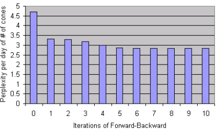
[image:7.612.313.532.586.684.2]Figure 13: IfT is the sequence of 34 training observations (33 days plusStop), thenp(T)increases rapidly during rees-timation. To compress the range of the graph, we don’t plot
p(T) but rather perplexity per observation= 1/34p
p(T) = 2−(log2p(T))/34.
nowHthat is used for the low-ice-cream midsummer days.) Should you care about this difference? As climatologists, you might very well be upset that the spreadsheet reversed cold and hot days. But sinceC
andHare ultimately just arbitrary labels, then per-haps the outcome is equally good in some sense. What does it mean for the outcome of this unsuper-vised learning procedure to be “good”? The dataset is just the ice cream diary, which makes no reference to weather. Without knowing the true weather, how can we tell whether we did a good job learning it?
10 Local Maximization of Likelihood
The answer: A good model is one that predicts the dataset as accurately as possible. The dataset actu-ally has temporal structure, since I tended to have long periods of high and low ice cream consump-tion. That structure is what the algorithm discov-ered, regardless of whether weather was the cause. The stateCorHdistinguishes between the two kinds of periods and tends to persist over time.
So did this learned model predict the dataset well? It was not always sure about the state sequence, but Figure 13 shows that the likelihood of the ob-served dataset (summed over all possible state se-quences) increased on every iteration. (Q: How is this found?30)
That behavior is actually guaranteed: repeated
30
It is the total probability of paths that explain the data, i.e., all paths in Figure 4, as given by column I of Figure 1; see footnote 10.
forward-backward reestimation converges to a local maximum of likelihood. We have already discov-ered two symmetric local maxima, both with per-plexity of 2.827 per day: the model might useCto represent cold andHto represent hot, or vice versa. Q: How much better is 2.827 than a model with no temporal structure?31
Remember that maximizing the likelihood of the training data can lead to overfitting. Q: Do you see any evidence of this in the final probability table?32 Q: Is there a remedy?33
11 A Trick Ending
We get very different results if we slightly mod-ify Figure 12 by putting p(1 | H) = 0.3 with
p(2 | H) = 0.4. The structure of the solution is very different (Figure 14). In fact, the final param-eters now show anti-inertia, giving a reconstruction similar to Figure 6b. Q: What went wrong?34
In the two previous local maxima, Hmeant “low ice-cream day” or “high ice-cream day.” Q: Accord-ing to Figure 14, what doesHmean here?35 Q: What does the low value ofp(H|H)mean?36
So we see that there are actually two kinds of structure coexisting in this dataset: days with a lot (little) ice cream tend to repeat, and days with 2 ice creams tend not to repeat. The first kind of structure did a better job of lowering the perplexity, but both
31A: A model with no temporal structure is a unigram model.
A good guess is that it will have perplexity 3, since it will be completely undecided between the 3 kinds of observations. (It so happens that they were equally frequent in the dataset.) How-ever, if we prevent the learning of temporal structure (by setting the initial conditions so that the model is always in stateC, or is always equally likely to be in statesCandH), we find that the perplexity is 3.314, reflecting the four-way unigram distribution
p(1) =p(2) =p(3) = 11/34, p(Stop)=1/34.
32A:p(H | Start) →1because we become increasingly
sure that the training diary started on a hot day. But this single training observation, no matter how justifiably certain we are of it, might not generalize to next summer’s diary.
33A: Smoothing the fractional counts. Note: If a prior is used
for smoothing, the algorithm is guaranteed to locally maximize the posterior (in place of the likelihood).
34
A: This is a third local maximum of likelihood, unrelated
to the others, with worse perplexity (3.059). Getting stuck in poor local maxima is an occupational hazard.
35
A:Husually emits 2 ice creams, whereasCnever does. So
Hstands for a 2-ice-cream day.
36
A: That 2 ice creams are rarely followed by 2 ice creams.
Figure 14: A suboptimal local maximum.
are useful. Q: How could we get our model to dis-cover both kinds of structure (thereby lowering the perplexity further)?37
Q: We have now seen three locally optimal mod-els in which the H state was used for 3 different things—even though we named itHfor “Hot.” What does this mean for the application of this algorithm to part-of-speech tagging?38
12 Follow-Up Assignment
In a follow-up assignment, students applied Viterbi decoding and forward-backward reestimation to part-of-speech tagging.39
In the assignment, students were asked to test their code first on the ice cream data (provided as a small tagged corpus) before switching to real data. This cemented the analogy between the ice cream and tagging tasks, helping students connect the class to the assignment.
37
A: Use more states. Four states would suffice to distinguish
hot/2, cold/2, hot/not2, and cold/not2 days.
38
A: There is no guarantee thatNandVwill continue to dis-tinguish nouns and verbs after reestimation. They will evolve to make whatever distinctions help to predict the word sequence.
39
Advanced students might also want to read about a mod-ern supervised trigram tagger (Brants, 2000), or the mixed re-sults when one actually trains trigram taggers by EM (Merialdo, 1994).
Furthermore, students could check their ice cream output against the spreadsheet, and track down basic bugs by comparing their intermediate results to the spreadsheet’s. They reported this to be very useful. Presumably it helps learning when students actually find their bugs before handing in the assignment, and when they are able to isolate their misconceptions on their own. It also made office hours and grading much easier for the teaching assistant.
13 Availability
The spreadsheet (in Microsoft Excel) and assign-ment are available at http://www.cs.jhu. edu/˜jason/papers/#tnlp02.
Also available is a second version of the spread-sheet, which uses the Viterbi approximation for de-coding and reestimation. The Viterbi algorithm is implemented in an unconventional way so that the two spreadsheets are almost identical; there is no need to follow backpointers. The probability of the best path through stateHon day 3 isµ3(H)·ν3(H),
whereµandνare computed likeαandβbut maxi-mizing rather than summing path probabilities. The Viterbi approximation treatsp3(H)as 1 or 0
accord-ing to whether µ3(H) ·ν3(H) equals max(µ3(C)·
ν3(C), µ3(H)·ν3(H)).
Have fun! Comments are most welcome.
References
L. E. Baum. 1972. An inequality and associated max-imization technique in statistical estimation of proba-bilistic functions of a Markov process. Inequalities, 3. Thorsten Brants. 2000. TnT: A statistical part-of-speech
tagger. In Proc. of ANLP, Seattle.
K. W. Church. 1988. A stochastic parts program and noun phrase parser for unrestricted text. Proc. of ANLP. Steven J. DeRose. 1988. Grammatical category
disam-biguation by statistical optimization. Computational
Linguistics, 14(1):31–39.
Jason Eisner. 2002. Parameter estimation for probabilis-tic finite-state transducers. In Proc. of ACL.
Steffen L. Lauritzen. 1995. The EM algorithm for graph-ical association models with missing data.
Computa-tional Statistics and Data Analysis, 19:191–201.
Bernard Merialdo. 1994. Tagging English text with a probabilistic model. Comp. Ling., 20(2):155–172. Judea Pearl. 1988. Probabilistic Reasoning in
Intelli-gent Systems: Networks of Plausible Inference.
Mor-gan Kaufmann, San Mateo, California.
L. R. Rabiner. 1989. A tutorial on hidden Markov mod-els and selected applications in speech recognition.