Towards Time Aware Knowledge Graph Completion

Towards Time-Aware Knowledge Graph Completion

Tingsong Jiang, Tianyu Liu, Tao Ge, Lei Sha, Baobao Chang, Sujian Li and Zhifang Sui

Key Laboratory of Computational Linguistics, Ministry of Education School of Electronics Engineering and Computer Science, Peking University Collaborative Innovation Center for Language Ability, Xuzhou 221009 China

{tingsong,tianyu0421,taoge,shalei,chbb,lisujian,szf}@pku.edu.cn

Abstract

Knowledge graph (KG) completion adds new facts to a KG by making inferences from existing facts. Most existing methods ignore the time information and only learn from time-unknown fact triples. In dynamic environments that evolve over time, it is important and challenging for knowledge graph completion models to take into account the temporal aspects of facts. In

this paper, we present a novel time-awareknowledge graph completion model that is able to

predict links in a KG using boththe existing facts andthe temporal information of the facts. To

incorporate the happening time of facts, we propose a time-aware KG embedding model using temporal order information among facts. To incorporate the valid time of facts, we propose a joint time-aware inference model based on Integer Linear Programming (ILP) using temporal consistency information as constraints. We further integrate two models to make full use of global temporal information. We empirically evaluate our models on time-aware KG completion task. Experimental results show that our time-aware models achieve the state-of-the-art on temporal facts consistently.

1 Introduction

Knowledge graphs (KGs) such as Freebase (Bollacker et al., 2008) and YAGO (Fabian et al., 2007) are extremely useful resources for many NLP related applications such as relation extraction and question answering, etc. Although KGs are large in size, they are far from complete (West et al., 2014). Knowl-edge graph completion, i.e., automatically inferring missing facts between entities in a knowlKnowl-edge graph, has thus become an increasingly important task. Recently a promising approach called KG embedding aims to embed the components (entities and relations) of a KG into a continuous vector space while preserving the inherent structure of a knowledge graph (Nickel et al., 2011; Bordes et al., 2011). This kind of approach has shown good effectiveness and scalability for KG completion.

However, most existing KG embedding models ignore the temporal information of facts. In the real

world, many facts are not static but highly ephemeral. For example, (Steve Jobs,diedIn, California)

happened on 2011-10-05; (Ronaldo,playsFor, A.C.Milan) is true only during 2007-2008. Intuitively,

temporal aspects of facts should play an important role when we perform KG completion. In this paper, we focus on time-aware KG completion. Specially, we incorporate two kinds of temporal information for

KG completion: (a)temporal order informationand (b)temporal consistency information. Bytemporal

order information, we mean that many facts have temporal dependencies on others according to the time

that they happened. For example, the facts involving a personPmay follow the following timeline: (P,

wasBornIn, )→(P,graduateFrom, )→(P,workAt, )→(P,diedIn, ). Given the time after

Pdied , it’s not proper to predict relations likeworkAt. Bytemporal consistency information, we mean

that many facts are only valid during a short time period. For example, a person’s marriage may be valid for a short period. Besides, the periods of a person’s different marriages should not overlap. Without considering the temporal aspects of facts, the existing KG embedding methods may make mistakes. It is also non-trivial for existing KG embedding methods to incorporate such temporal information.

This work is licenced under a Creative Commons Attribution 4.0 International Licence. Licence details: http://creativecommons.org/licenses/by/4.0/

To deal with the issues of the existing KG embedding methods, we propose twotime-aware KG com-pletionmodels to incorporate the above two kinds of temporal information, respectively. The extensive experimental results show the effectiveness of the two proposed models. We further propose a joint model that achieves better results. Our contributions include the following:

• To the best of our knowledge, this is the first work for time-aware KG completion. To incorporate

the temporal order information, we propose a novel time-aware embedding (TAE) model that en-codes the temporal order information as a regularizer on the geometric structure of the embedding space. To incorporate more temporal consistency information, we propose using Integer Linear Programming (ILP) to encode the temporal consistency information as constraints.

• We further propose a joint framework to unify the two complementary time-aware models

seamless-ly. ILP model considers more temporal constraints than TAE model, while TAE model generates more accurate embeddings for the objective function of ILP model. Our framework can be general-ized to many KG embedding models such as TransE (Bordes et al., 2013) model and its extensions.

• We create real-world temporal data sets based on YAGO2 and Freebase for time-aware KG

com-pletion. The evaluation results show that our models outperform the start-of-the-art approaches and it confirms the effectiveness of incorporating temporal information.

The rest of the paper is organized as follows. Section 2 and Section 3 describe two time-aware KG completion models, respectively. Experiments, related work and conclusion are shown in Section 4-6. 2 Time-Aware KG Embedding Model

Time-aware KG embedding aims to automatically learn entity and relation embeddings by exploiting both observed triple facts and temporal order information among facts.

2.1 Time-Aware KG Completion Task

We represent facts with temporal annotations by quadruples, quads for short. We use(ei, r, ej, t) to

denote the fact thatei andej has relationrduring the time interval t= [tb, te]withtb < te. Although

our reasoning framework supports arbitrary continuous intervals over real number, for simplicity, we

assume time intervals range overyears. For example, the interval [1980, 1999] starts in 1980 and ends

in 1999. For some facts that happened at a certain time and did not last, we havetb=te. For some facts

that does not end yet, we representtast= [tb,+∞].

KG completion is the task of predicting whether a given edge (ei, r, ej) exists in the graph or not.

However, most facts are time-dependent and hold only for a given time period. For example, the fact of George W. Bush’s presidency is only meaningful from 2001 to 2009. To incorporate temporal informa-tion for a more accurate representainforma-tion, we extend this task to include the time dimension of the facts and call ittime-aware KG completion, i.e., to complete the quad(ei, r, ej, t)whenei,rorej is missing

given a specific time intervalt. For example, we can answer the question“Who is the president of USA

in 2010?”by predicting head entity in(?,presidentOf, USA, [2010,2010]).

2.2 Traditional KG Embedding Methods

Traditional KG embedding methods use only the observed time-unknown facts (triples) to learn entity and relation representations. TransE (Bordes et al., 2013) is an efficient and simple model among them.

The basic idea behind TransE is that the relation between two entities ei,ej ∈ Rn corresponds to a

translation vectorr∈Rn_{between them, i.e.,ei+r≈ej when(ei, r, ej)holds. The scoring function is}

defined as measuring its plausibility in the vector space:

f(ei, r, ej) =kei+r−ejk`1/`2, (1)

wherek · k_`1/`2 denotes the`1-norm or`2-norm. A margin-based ranking loss is optimized to derive the

entity and relation representations:

min X

x+_∈∆ X

x−_∈∆0

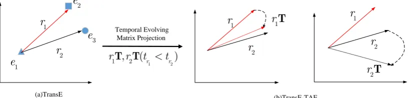
Temporal Evolving

Figure 1: Simple illustration of Temporal Evolving MatrixT in the time-aware embedding (TAE)

s-pace. For example,r1=wasBornInhappened before r2=diedIn. After projection byT, we get prior

relation’s projectionr1Tnear subsequent relationr2 in the space, i.e.,r1T≈r2, butr2T6=r1.

Here,x+ _{∈ ∆is the observed (i.e., positive) triple, and x}−_∈∆0 _{is the negative triple constructed by} replacing entities inx+_{. γ is the margin separating positive and negative triples and[z]+ = max(0, z).}

Please refer to (Wang et al., 2014a; Lin et al., 2015b) for TransH, TransR and other models.

After we obtain the embeddings, the plausibility of a missing triple can be predicted by using the scoring function. In general, triples with higher plausibility are more likely to be true.

2.3 Time-Aware KG Embedding Model

TransE assumes that each relation is time independent and entity/relation representation is only affect-ed by structural patterns in KGs. To better model knowlaffect-edge evolution, we assume temporal orderaffect-ed relations are related to each other and evolve in a time dimension. For example, for the same person,

there exists a temporal order among relationswasBornIn→graduatedFrom→diedIn. In time

dimension, wasBornIncan evolve into graduateFromanddiedIn, but diedIncannot evolve

intowasBornIn.

To compare temporal orders, we define a pair of temporal ordering relations sharing the same head

entity 1 _{astemporal ordering relation pair, e.g., hwasBornIn, diedIni. We define the relation}

happening earlier, e.g.,wasBornIn, asprior relationand the other assubsequent relation. We define

hprior relation, subsequent relationias positive temporal ordering pairs andhsubsequent relation, prior relationias negative ones.

To capture the temporal order of relations, we further define atemporal evolving matrixT ∈ Rn×n

to model relation evolution, where nis the dimension of relation embedding. T is a parameter to be

learned by the model from the data. We assume that prior relation can evolve into subsequent relation through the temporal evolving matrix. The more frequent they have temporal orders, the more they can evolve. Specially, as in Figure 1, prior relationr1 projected byTshould be near subsequent relationr2,

i.e.,r1T≈r2, whiler2Tshould be far fromr1. In this way, we are able to separate prior relation and

subsequent relation automatically during training.

We formulate time-aware KG completion as an optimization problem based on a regularization ter-m. Given any positive training quad (ei, rk, ej, trk) ∈ ∆t, we can find a temporally related quad

(ei, rl, em, trl) ∈ ∆t sharing the same head entity and a temporal ordering relation pair hrk, rli. If trk<trl, we have a positive temporal ordering relation pairy+ =hrk, rliand the corresponding negative

relation pairy− _{= hr}

k, rli−1 = hrl, rkiby inverse. Our optimization requires that positive temporal

ordering relation pairs should have lower scores (energies) than negative pairs. Therefore, we define a

temporalscoring function as

g(hrk, rli) =krkT−rlk`1/`2, (3)

which is expected to give a low score when the temporal ordering relation pair is in chronological order,

and a high score otherwise. Note thatTis asymmetric and the loss function is also asymmetric so as to

capture temporal order information.

To make the embedding space compatible with the observed triples, we make use of the fact triples set

∆and follow the same strategy adopted in previous methods. Specially, we apply the samefactscoring

functionf(ei, rk, ej)in Equation (1) to each candidate triple. The optimization is to minimize thejoint

scoring function,

by replacing entities. The positive temporal ordering relation pair set with respect to(ei, rk, ej, trk)is

defined as

Ωei,trk ={hrk, rli|(ei, rk, ej, trk)∈∆t,(ei, rl, em, trl)∈∆t, trk< trl}

∪{hrl, rki|(ei, rk, ej, trk)∈∆t,(ei, rl, em, trl)∈∆t, trk> trl}

(5)

where rk and rl share the same head entity ei. Ω0ei,t_rk are the corresponding negative relation pairs

by inverse the relation pairs. In experiments, our constrains are keik2 ≤ 1, krkk2 ≤ 1, krlk2 ≤ 1, kejk2≤1,krkTk2≤1, andkrlTk2≤1to avoid overfitting similarly to previous work.

The first term in Equation (1) enforces the generated embedding space compatible with all the observed triples, and the second term further requires the space to be temporally consistent and more accurate.

Hyperparameterλstrikes a trade-off between the two cases. Stochastic gradient descent (in mini-batch

mode) is adopted to solve the minimization problem.

3 Joint Inference for Time-Aware KG Completion

In this section, we incorporate temporal information as temporal consistency constraints for KG comple-tion. We take advantage of temporal logic transitivity and use ILP to derive more accurate predictions.

3.1 Temporal Consistency Constraints

The candidate predictions we obtained in the traditional KG embedding inevitably include many incor-rect predictions. By applying temporal consistency constraints, we can identify and then discard such errors to produce more accurate results.

As the complexity of resolving conflicts strictly depends on the constraints to apply, we need to choose them with great care. In the following, we consider three kinds of temporal constraints.

Temporal Disjointness. The time intervals of any two facts with a common functional relation and a common head entity are non-overlapping. For example, a person can only be spouse of one person at a time:(e1,wasSpouseOf, e2,[1990,2010))∧(e1,wasSpouseOf, e3,[2005,2013))∧e26=e3→false.

Temporal Ordering. For some temporal ordering relations, one fact always happens before

an-other fact. For example, a person must be born before he graduated: (e1,wasBornIn, e2, t1) ∧

(e1,graduateFrom, e3, t2)∧t1> t2→false.

Temporal Spans.Some facts are true only during a specific time span. In general, the fact is invalid for other time periods outside the range of its time span in KGs. For example, given time intervalt0_outside the rangetin(e1,presidentOf, e2, t)∈KG, the fact(e1,presidentOf, e2, t0)is invalid.

3.2 Integer Linear Program Formulation

We formulate the time-aware inference as an ILP problem with temporal constraints. Traditional KG embedding methods can capture the intrinsic properties of data, which can be treated as a probability to predict unseen facts. For each candidate fact (ei, rk, ej), we use w_ij(k) = f(ei, rk, ej) to represent

the plausibility predicted by an embedding model, and introduce a Boolean decision variable x(_ijk) to

indicate whether the fact(ei, rk, ej, t) is true or not for timet. Our aim is to find the best assignment

to the decision variables, maximizing the overall plausibility while complying with all the temporal constraints. The objective function can be written as:

maxX

x(ijk)

w_ij(k)x(_ijk). (6)

The temporal disjointness constraints avoid the disagreement between the predictions of two facts sharing the same head entity and relation. These constraints can be represented as:

x(_ijk)+x(_ilk)≤1,∀k∈ Cd, t_x(k)

ij ∩tx(ilk) 6=∅ (7)

whereCd_{are functional relations described such aswasSpouseOfandt}

x(_ijk), tx(_ilk) are time intervals for

two facts, respectively.

The Temporal Ordering constraints ensure the occurring order for some relation pairs. These con-straints can be represented as:

x(_ijk)+x_il(k0)≤1,∀(k, k0_{)∈ C}o_{, t}

x(_ijk) ≥tx(_ilk) (8)

whereCo _{= {hr}

k, rk0i}are relation pairs that have precedent orders such ashwasBornIn,diedIni.

These relation pairs are discovered automatically in the training set by statistics and finally manually calibrated.

The temporal span constraints ensure the specific time span when the corresponding fact is true. These constraints can be represented as:

x(_ijk)= 0,∀k∈ Cs_{, t}

x(_ijk) ∩t∆=∅ (9)

whereCs _{are those relations valid for only a specific time span such aspresidentOfandt}

∆is the

valid time span in KG.

Using ILP, we can combine the ability of capturing the intrinsic properties of KG data and the temporal constraints that are embedded into global consistencies of the relations together. As shown in Eq.(10),

any unseen fact’s plausibility is encoded in scores wk

ij which captures the intrinsic properties of KG

data. Temporal consistency constraints are formulated as Eq.(7)-(9) and apply to the objective function naturally. By solving Eq.(10), we will obtain a list of selected candidate entities or relations for a missing fact as our final output.

3.3 Integrating Two Time-Aware Models

As mentioned above, the two time-aware models are complementary for each other: ILP model considers more temporal constraints than TAE model while TAE model generates more accurate embeddings for the ILP objective function.

For each unseen quad(ei, rk, ej, t), we use a Boolean decision variablex(ijk,t)to indicate whether it’s

true or not. We can use the embeddings of TAE model in Section 2.3 to calculate the plausibilityv_ij(k,t)

for the ILP objective function. The objective function is

max X

x(_ijk,t)

v_ij(k,t)x(_ijk,t). (10) Eq.(7)-(9) remain the same.

4 Experiments

We use similar evaluation metrics as traditional KG completion methods (Bordes et al., 2013) for time-aware KG completion.

4.1 Data Sets

To create temporal KG data sets, we need to decide whether a fact has temporal information. We catego-rize relations into time-sensitive relations and time-unsensitive relations according to YAGO2 (Hoffart

et al., 2013). For example,diedInis time-sensitive, buthasNeighboris not. We extract temporal

annotations for time-sensitive facts from YAGO2 and Freebase2_.

In YAGO2, temporal facts are in the form (factID,occurSince,tb), (factID,occurUntil,te) indicating

the fact is true during[tb, te]. HerefactIDdenotes a specific fact(ei, r, ej). We directly represent these

temporal facts as quads(ei, r, ej,[tb, te]). We selected 10 frequent time-sensitive relations to make a pure

temporal data set. Then we selected the subset of entities which have at least two mentions in temporal

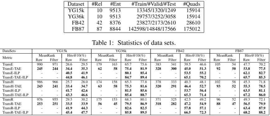
Dataset #Rel #Ent #Train/#Valid/#Test #Quads

Metric _RawMeanRank_{Filter Raw}Hits@10(%)_{Filter Raw}MeanRank_{Filter Raw}Hits@10(%)_{Filter Raw}MeanRank_{Filter Raw}Hits@10(%)_{Filter Raw}MeanRank_{Filter Raw}Hits@10(%)_Filter

TransE 990 971 26.6 29.5 179 163 65.7 75.6 383 341 39.5 46.6 105 54 47.7 70.2

TransE-TAE 245 244 34.4 35.3 62 58 75.4 81.9 328 300 45.0 51.3 92 50 53.8 77.5

TransE-ILP - - 40.5 41.9 - - 80.1 85.4 - - 53.5 55.2 - - 62.1 82.7

TransE-TAE-ILP - - 44.8 46.1 - - 84.7 89.4 - - 65.1 70.2 - - 65.7 85.3

TransH 986 966 25.7 28.0 174 158 65.3 77.8 378 333 40.3 48.1 102 58 45.3 71.8

TransH-TAE 243 241 33.4 34.7 63 58 75.3 81.6 320 291 46.4 52.7 93 52 55.3 78.5

TransH-ILP - - 41.7 42.6 - - 81.5 85.6 - - 53.7 56.4 - - 63.5 81.1

TransH-TAE-ILP - - 43.3 46.6 - - 85.4 88.7 - - 65.3 71.4 - - 67.2 86.0

TransR 976 955 29.5 30.2 175 153 68.3 80.1 371 325 42.5 49.2 96 52 49.3 72.1

TransR-TAE 253 251 33.5 33.9 56 45 79.5 86.9 318 282 47.2 54.9 88 47 56.5 79.9

TransR-ILP - - 41.9 44.3 - - 82.6 82.5 - - 57.8 57.1 - - 63.4 87.9

TransR-TAE-ILP - - 45.4 47.7 - - 85.8 89.5 - - 66.5 72.3 - - 68.2 88.2

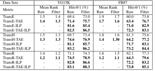
Table 2: Evaluation results on entity prediction.

facts. This resulted in 15,914 triples (quadruples) which were randomly split with the ratio shown in

Table 1. This data set is denotedYG15k. Although YAGO2 has many temporal annotations for facts,

a lot of temporal annotations are still missing for time-sensitive facts. We consider the data setYG36k

consisting of half facts with temporal annotations and the other half missing temporal annotations to evaluate whether partial temporal information of data improves the performance or not. The relationship set is the same in YG15k and YG36k.

We extracted temporal facts mainly from FB15k (Bordes et al., 2013), a subset of Freebase consisting of 1345 relations. Among them, 707 relations are long relations in the form“r1.r2”concatenating short

relationsr1andr2. Long relations do not exist in the original schema of Freebase. Many associated facts

in Freebase are organized as a CVT structure (similar to an event), e.g., (Einstein,hasWonPrize,

No-bel) is stored as (Einstein,/award/award winner/awards won,x), (x,/award/award honor/award,Nobel)

in Freebase, wherexis calledmediatorand not a real entity. FB15k facts are created by concatenating

two relations: (Einstein,/award/award winner/awards won. /award/award honor/award,Nobel). We

ex-tracted temporal annotations from the original Freebase CVT structure for these facts with long relations. For short relations such as/film/director/film, we used creation/destruction dates of head or tail entity as their time, e.g., the released date of the film. This resulted in 42 time-sensitive relations and 28,610

temporal facts. We denoted the data set as FB42. We further added triples without time annotations

and created FB87. In FB15k, there are about 50% temporal facts in our setting. The data set will be

publicly available. All experiments are repeated five times by drawing new training/validation/test splits, and results averaged over the five rounds are reported.

4.2 Time-aware KG Completion

Time-aware KG completion (link prediction) is to complete the triple (ei, r, ej, t) when ei, r or ej is

missing given a specific time intervalt. We divided the stage into two sub-tasks, i.e., entity prediction and relation prediction.

4.2.1 Entity Prediction

Evaluation protocol. For each test triple with missing head or tail entity, various methods are used to compute the scores for all candidate entities and rank them in descending order. We use two metrics for our evaluation as in (Bordes et al., 2013): the mean of correct entity ranks (Mean Rank) and the proportion of valid entities ranked in top-10 (Hits@10). As mentioned in (Bordes et al., 2013), the metrics are desirable but flawed when a corrupted triple exists in the KG. As a countermeasure, we may filter out all these corrupted triples which have appeared in KG before ranking. We name the first evaluation set asRawand the second asFilter.

For each test quad (triple), we replace the head/tail entity ei by those entities with compatible types

Wang et al., 2015). Entity type information is easy to obtain for YAGO and Freebase. Then we rank the generated corrupted triples in descending order, according to the plausibility (for baselines and TAE model) or the decision variables (for time-aware ILP model). Then we check whether the original cor-rect triple ranks in top-10. To calculate Hit@10 for ILP model, for each test quad, we add additional constraints that at most 10 corrupted are true: P_i,jx(r1)

eiej ≤10. Mean Rank is missing for ILP method

as we could not rank the binary decision variables.

Baseline methods.For comparison, we select TransE (Bordes et al., 2013), its extensions TransH (Wang et al., 2014b) and TransR (Lin et al., 2015b) as our baselines. We then compare time-aware embedding and time-aware ILP inference with each baseline. For example, TransE with TAE and time-aware ILP is denoted as “TransE-TAE” and “TransE-ILP”, respectively. The combined model of the two time-aware models are denoted as “TransE-TAE+ILP”.

Implementation details. For all embedding methods, we create 100 mini-batches on each data set. The dimension of the embeddingnis set in the range of{20,50,100}, the marginγ1andγ2are set in the range {1,2,4,10}. The learning rate is set in the range{0.1, 0.01, 0.001}. The regularization hyperparameter

λis tuned in{10−1_,10−2_,10−3_,10−4_{}. The best configuration is determined according to the mean rank}

in validation set. For YAGO data set, the optimal configurations aren= 100,γ1 =γ2 = 4,λ= 10−2,

learning rate is 0.001 and taking`1−norm; For Freebase data set, the optimal configurations are n =

100,γ1 =γ2 = 1,λ= 10−1, learning rate is 0.001 and taking`1−norm.

We then incorporate temporal constraints into the six models with optimal parameter settings using ILP. To generate the objective function of ILP, plausibility predicted by embedding models is normalized byw0

ij = (wij −MIN)/(MAX−MIN), where MAXand MINare max/min scores for each corrupted

test triple. We use the lp solve package3_{to solve the ILP problem.}

Results. Table 2 reports the results for each data set. From the results, we can see that 1) TAE methods outperform all the baselines on all the data sets and with all the metrics. The improvements are quite sig-nificant. The Mean Rank drops by about 75%, and Hits@10 rises about 19% to 30%. This demonstrates the superiority and generality of our method. 2) Adding more temporal facts improve the performance for TAE models. YG15k consists of 100% temporal facts while YG36k consists of 50% temporal facts. All the temporal information in YG15k is utilized to model temporal associations and make the embed-dings more accurate. Therefor, it obtains larger improvement for TAE than YG36k. 3) Improvement for YAGO is larger than Freebase because YAGO data set contains more temporal ordering relation pairs than Freebase data set.

As we can see from Table2, the time-aware ILP method improves each baseline model by about 10% to 16%. This demonstrates the effectiveness of incorporating temporal consistency constraints. Combining two time-aware models further improves the performance by 2% to 3%. This indicates that 1) although TAE models encode temporal order information, only pair-wise temporal ordering relations are optimized during each training iteration. ILP can take advantage of global temporal transitivity which pair-wise methods can’t. 2) Adding time span information in the ILP model can remove more false predictions.

4.2.2 Relation Prediction

Relation prediction aims to predict relations between two entities. Evaluation results are shown in Table 3 on YG15K and FB87 due to space limit, and here we report Hits@1 instead of Hits@10. For ILP models, we report Hits@1 for the same reason in entity prediction. Again, two time-aware models improve baselines greatly.

The ILP models improve the precision by about 10%, showing that incorporating temporal constraints directly is better for this task. The main reason is that our temporal constraints are designed to better han-dle temporal conflicts in relations. Relation prediction and relation extraction from text have common

multi-label problems that the same entity pair may have multiple relation labels. For example,

(Oba-ma,US)could have two valid relations: wasPresidentOf, wasBornIn. Through temporal constraints, we are aware that the two relations have different valid time, and therefore we could remove the false one to

Data Sets YG15K FB87

Metric _RawMean Rank_{Filter Raw}Hits@1 (%)_{Filter Raw}Mean Rank_{Filter Raw}Hits@1 (%)_Filter TransE 1.5 1.4 69.4 73.0 1.9 1.7 60.0 73.8 TransE-TAE 1.4 1.3 71.4 75.7 1.7 1.6 63.4 76.7 TransE-ILP - - 81.6 85.4 - - 71.0 82.9 TransE-TAE-ILP - - 82.5 86.5 - - 72.3 83.1 TransH 1.5 1.3 69.7 73.4 1.8 1.6 61.3 75.6 TransH-TAE 1.3 1.3 74.6 76.9 1.4 1.30 64.2 77.2 TransH-ILP - - 81.1 85.7 - - 71.7 83.1 TransH-TAE-ILP - - 83.2 86.2 - - 73.2 84.4 TransR 1.4 1.2 71.1 74.3 1.6 1.5 62.1 77.3 TransR-TAE 1.2 1.1 74.5 78.9 1.2 1.1 64.3 79.6 TransR-ILP - - 82.8 86.6 - - 72.2 83.2 TransR-TAE-ILP - - 83.1 88.3 - - 73.8 85.1

Table 3: Evaluation results on relation prediction.

Testing quads TransE TransE-TAE TransE-ILP

(Stanford Moore,?,New York City,[1982,1982]) wasBornIn,diedIn diedIn,wasBornIn diedIn,wasBornIn

(John Schoenherr,?,Caldecott Medal,[1988,1988]) owns,hasWonPrize hasWonPrize,created hasWonPrize,created

(John G. Thompson,?,University of Cambridge,[1968,1994]) graduatedFrom,worksAt worksAt,graduatedFrom worksAt,graduatedFrom (Tommy Douglas,?,New Democratic Party,[1961,1972]) isMarriedTo,isAffiliatedTo isAffiliatedTo,isMarriedTo isAffiliatedTo,isMarriedTo (Carmen Electra,?,Owen Wilson,[2004,2005]) isMarriedTo,sameAward winner isMarriedTo,sameAward winner sameAward winner,isMarriedTo

Table 4: Examples of relation prediction in descending order. Correct predictions are inbold.

improve Hit@1 accuracy.

Qualitative analysis.Examples of relation prediction for TransE, TransE-TAE and TransE-ILP are com-pared in Table 4. From the results we have the following two conclusions. 1) Temporal order information is useful to distinguish similar relations. For example, when testing(Stanford Moore, ? , Chicago, [1982, 1982]), it’s easy for TransE to mix relationswasBornInanddiedInas they behave similarly for a

per-son and a place. But knowing that hegraduatedin 1935 from the training set, and TransE-TAE have

learnt temporal order thatwasBornIn→graduated→diedIn, the regularization term|rgraduateT−rdied|

and|rgraduateT−rborn|helps rankdiedInhigher thanwasBornIn. TransE-ILP also benefits from

such temporal order constraints and obtains more accurate predictions. 2) Time span information is

useful to make accurate predictions. For example, TransE and TransE-TAE both predict (Carmen

Elec-tra,?,Owen Wilson,[2004,2005]) haswasMarriedTorelation. Temporal order constraints don’t work

for this example. But the time span constraints help TransE-ILP to removewasMarriedTobecause

Carmen Electrawas married toDave Navarroduring [2003,2008] and a person cannot marry two people at the same time.

5 Related Work

There are two lines of research related to our work.

Knowledge Graph Completion. Nickel et al. (2016) provide a broad overview of machine learning models for KG completion. These models predict new facts in a given knowledge graph using informa-tion from existing entities and relainforma-tions. The most related work from this line of work is KG embedding models (Nickel et al., 2011; Bordes et al., 2013; Socher et al., 2013). Aside from fact triples, external information is employed to improve KG embedding such as combining text (Riedel et al., 2013; Wang et al., 2014a; Zhao et al., 2015), entity type and relationship domain (Guo et al., 2015; Chang et al., 2014), relation path (Lin et al., 2015a; Gu et al., 2015), and logical rules (Wang et al., 2015; Rockt¨aschel et al., 2015). However, these methods have not utilized temporal information among facts.

6 Conclusion and Future Work

In this paper, we propose two novel time-aware KG completion models. Time-aware embedding (TAE) model imposes temporal order constraints on the geometric structure of the embedding space and en-forces it to be temporally consistent and accurate. Time-aware joint inference with ILP framework considers global temporal constraints as well as KG embeddings. It naturally preserves the benefits of embedding models and is more accurate with respect to various temporal constraints. We further inte-grate two models to make full use of temporal information.

As future work: 1) Many temporal facts are not stored by current KGs (about 30% facts in YAGO and 50% in Freebase lack temporal annotations), we will extract more temporal information from texts. 2) We will consider using our time-aware KG completion model to predict temporal scopes of new facts. Acknowledgements

This research is supported by National Key Basic Research Program of China (No.2014CB340504) and National Natural Science Foundation of China (No.61375074,61273318). The contact author for this paper are Baobao Chang and Zhifang Sui.

References

Javier Artiles, Qi Li, Taylor Cassidy, Suzanne Tamang, and Heng Ji. 2011. Cuny blender tackbp2011 temporal

slot filling system description. InProceedings of Text Analysis Conference (TAC).

Steven Bethard and James H Martin. 2007. Cu-tmp: Temporal relation classification using syntactic and

se-mantic features. InProceedings of the 4th International Workshop on Semantic Evaluations, pages 129–132.

Association for Computational Linguistics.

Kurt Bollacker, Colin Evans, Praveen Paritosh, Tim Sturge, and Jamie Taylor. 2008. Freebase: a collaboratively

created graph database for structuring human knowledge. InProceedings of the 2008 ACM SIGMOD

interna-tional conference on Management of data, pages 1247–1250. ACM.

Antoine Bordes, Jason Weston, Ronan Collobert, and Yoshua Bengio. 2011. Learning structured embeddings of

knowledge bases. InConference on Artificial Intelligence, number EPFL-CONF-192344.

Antoine Bordes, Nicolas Usunier, Alberto Garcia-Duran, Jason Weston, and Oksana Yakhnenko. 2013.

Trans-lating embeddings for modeling multi-relational data. InAdvances in Neural Information Processing Systems,

pages 2787–2795.

Taylor Cassidy, Bill McDowell, Nathanael Chambers, and Steven Bethard. 2014. An annotation framework for

dense event ordering. InACL.

Nathanael Chambers and Daniel Jurafsky. 2008. Unsupervised learning of narrative event chains. ACL,

94305:789–797.

Nathanael Chambers, Shan Wang, and Dan Jurafsky. 2007. Classifying temporal relations between events. In

Proceedings of the 45th Annual Meeting of the ACL on Interactive Poster and Demonstration Sessions, pages 173–176. Association for Computational Linguistics.

Kai-Wei Chang, Wen-tau Yih, Bishan Yang, and Christopher Meek. 2014. Typed tensor decomposition of

knowl-edge bases for relation extraction. InEMNLP, pages 1568–1579.

Maximilian Dylla, Mauro Sozio, and Martin Theobald. 2011. Resolving temporal conflicts in inconsistent rdf

knowledge bases. InBTW, pages 474–493.

MS Fabian, K Gjergji, and W Gerhard. 2007. Yago: A core of semantic knowledge unifying wordnet and

wikipedia. In16th International World Wide Web Conference, WWW, pages 697–706.

Guillermo Garrido, Anselmo Penas, Bernardo Cabaleiro, and Alvaro Rodrigo. 2012. Temporally anchored relation

extraction. InProceedings of the 50th Annual Meeting of the Association for Computational Linguistics: Long

Papers-Volume 1, pages 107–116. Association for Computational Linguistics.

Kelvin Gu, John Miller, and Percy Liang. 2015. Traversing knowledge graphs in vector space. arXiv preprint

Shu Guo, Quan Wang, Bin Wang, Lihong Wang, and Li Guo. 2015. Semantically smooth knowledge graph

embedding. InProceedings of the 53rd Annual Meeting of the Association for Computational Linguistics and

the 7th International Joint Conference on Natural Language Processing, pages 84–94.

Johannes Hoffart, Fabian M Suchanek, Klaus Berberich, and Gerhard Weikum. 2013. Yago2: A spatially and

temporally enhanced knowledge base from wikipedia. Artificial Intelligence, 194:28–61.

Yankai Lin, Zhiyuan Liu, and Maosong Sun. 2015a. Modeling relation paths for representation learning of

knowledge bases. arXiv preprint arXiv:1506.00379.

Yankai Lin, Zhiyuan Liu, Maosong Sun, Yang Liu, and Xuan Zhu. 2015b. Learning entity and relation embeddings for knowledge graph completion.

Xiao Ling and Daniel S Weld. 2010. Temporal information extraction. InAAAI, volume 10, pages 1385–1390.

Maximilian Nickel, Volker Tresp, and Hans-Peter Kriegel. 2011. A three-way model for collective learning on

multi-relational data. In Proceedings of the 28th international conference on machine learning (ICML-11),

pages 809–816.

Maximilian Nickel, Kevin Murphy, Volker Tresp, and Evgeniy Gabrilovich. 2016. A review of relational machine

learning for knowledge graphs. Proceedings of the IEEE, 104(1):11–33.

James Pustejovsky and Marc Verhagen. 2009. Semeval-2010 task 13: evaluating events, time expressions, and

temporal relations (tempeval-2). InProceedings of the Workshop on Semantic Evaluations: Recent

Achieve-ments and Future Directions, pages 112–116. Association for Computational Linguistics.

Sebastian Riedel, Limin Yao, Andrew McCallum, and Benjamin M Marlin. 2013. Relation extraction with matrix factorization and universal schemas.

Tim Rockt¨aschel, Sameer Singh, and Sebastian Riedel. 2015. Injecting logical background knowledge into

em-beddings for relation extraction. InProceedings of the 2015 Human Language Technology Conference of the

North American Chapter of the Association of Computational Linguistics.

Richard Socher, Danqi Chen, Christopher D Manning, and Andrew Ng. 2013. Reasoning with neural tensor

networks for knowledge base completion. InAdvances in Neural Information Processing Systems, pages 926–

934.

Partha Pratim Talukdar, Derry Wijaya, and Tom Mitchell. 2012a. Acquiring temporal constraints between

rela-tions. InCIKM.

Partha Pratim Talukdar, Derry Wijaya, and Tom Mitchell. 2012b. Coupled temporal scoping of relational facts. In

Proceedings of the fifth ACM international conference on Web search and data mining, pages 73–82. ACM. Yafang Wang, Mohamed Yahya, and Martin Theobald. 2010. Time-aware reasoning in uncertain knowledge

bases. InMUD, pages 51–65. Citeseer.

Yafang Wang, Bin Yang, Lizhen Qu, Marc Spaniol, and Gerhard Weikum. 2011. Harvesting facts from textual

web sources by constrained label propagation. In Proceedings of the 20th ACM international conference on

Information and knowledge management, pages 837–846. ACM.

Zhen Wang, Jianwen Zhang, Jianlin Feng, and Zheng Chen. 2014a. Knowledge graph and text jointly embedding. In Proceedings of the 2014 Conference on Empirical Methods in Natural Language Processing (EMNLP)., pages 1591–1601.

Zhen Wang, Jianwen Zhang, Jianlin Feng, and Zheng Chen. 2014b. Knowledge graph embedding by translating

on hyperplanes. InProceedings of the Twenty-Eighth AAAI Conference on Artificial Intelligence, pages 1112–

1119.

Quan Wang, Bin Wang, and Li Guo. 2015. Knowledge base completion using embeddings and rules. In

Proceed-ings of the 24th International Joint Conference on Artificial Intelligence, pages 1859–1865.

Robert West, Evgeniy Gabrilovich, Kevin Murphy, Shaohua Sun, Rahul Gupta, and Dekang Lin. 2014.

Knowl-edge base completion via search-based question answering. InProceedings of the 23rd international conference

on World wide web, pages 515–526. ACM.

Yu Zhao, Zhiyuan Liu, and Maosong Sun. 2015. Representation learning for measuring entity relatedness with

rich information. InProceedings of the 24th International Conference on Artificial Intelligence, pages 1412–