Contrasting Vertical and Horizontal Transmission of Typological Features
Kenji Yamauchi Yugo Murawaki
Graduate School of Informatics, Kyoto University Yoshida-honmachi, Sakyo-ku, Kyoto, 606-8501, Japan
yamauchi@nlp.ist.i.kyoto-u.ac.jp murawaki@i.kyoto-u.ac.jp
Abstract
Linguistic typology provides features that have a potential of uncovering deep phylogenetic re-lations among the world’s languages. One of the key challenges in using typological features for phylogenetic inference is that horizontal (spatial) transmission obscures vertical (phylogenetic) signals. In this paper, we characterize typological features with respect to the relative strength of vertical and horizontal transmission. To do this, we first construct (1) a spatial neighbor graph of languages and (2) a phylogenetic neighbor graph by collapsing known language families. We then develop an autologistic model that predicts a feature’s distribution from these two graphs. In the experiments, we managed to separate vertically and/or horizontally stable features from unstable ones, and the results are largely consistent with previous findings.
1 Introduction
Centuries of research in historical linguistics have identified groups of languages deriving from single common ancestors. Each of these groups, called a language family, is organized as a tree that reflects its evolutionary history. Such language families include Indo-European, Austronesian and Bantu languages. Despite the huge success, historical linguistics fails to link some languages with others, and hence they are called language isolates. For example, Basque, Burushaski and Japanese have no established relatives. Although there are several attempts to uncover deep phylogenetic relations, in which the results are often represented asmacrofamilies, they remain controversial (Dolgopolsky, 1998; Greenberg, 2000). We argue that the limitation of the mainstream approach is that it relies on lexical traits. Language families are established by demonstrating that its member languages sharecognates, or words that have a common etymological origin.1Lexical data are also the main target of modern statistical methods that are typically used to date the common ancestor (Swadesh, 1971; Gray and Atkinson, 2003). Language isolates are called so exactly because they lack reliable cognates.
For this reason, we follow a different line to research that makes use of typological data for phyloge-netic inference (Tsunoda et al., 1995; Dunn et al., 2005; Teh et al., 2008; Longobardi and Guardiano, 2009; Murawaki, 2015). Linguistic typology is a cross-linguistic study that classifies the world’s lan-guages according to structural properties such as basic word order (SVO, SOV, etc.) and the presence or absence of tone. On the one hand, typological features, by definition, allow us to compare an arbitrary pair of languages including language isolates. On the other hand, they pose several new challenges to us. While the sharing of cognates is a direct indicator of shared ancestry, the sharing of the same basic word order SOV, for example, is only a weak signal because it occurred multiple times in multiple places. We believe that computer-intensive statistical methods can help taming the inherent uncertainty.
In this paper, we give a step forward toward typology-based phylogenetic inference. We specifically tackle the problem that horizontal (spatial) transmission obscures vertical (phylogenetic) signals. Like
This work is licensed under a Creative Commons Attribution 4.0 International License. License details: http:// creativecommons.org/licenses/by/4.0/
1In historical linguistics, cognates are distinguished from loanwords. We broadly refer to both the traditionalcomparative methodand modern statistical methods as lexicon-based approaches because they require cognate identification. Note that historical linguists often use regular sound changes, in addition to cognates themselves, as features to determine the relative order of multiple branching events (Pellard, 2009).
Figure 1: Map of languages in WALS.
loanwords, typological features can be borrowed from one language to another. In fact, non-tree-like evolution has been one of the central topics in linguistic typology (Trubetzkoy, 1928). Lexicon-based approaches, especially statistical ones, often address this problem by narrowing the scope tobasic vo-cabulary,or a list of basic concepts. Words on the list are assumed to be resistant to borrowing (Swadesh, 1971), and some are even claimed to be extremely stable (Pagel et al., 2013). By contrast, typological features, in their original forms, are a mosaic with varying degrees of resistibility. We need to start with quantitatively characterizing each typological feature in this respect.
We present a probabilistic model that directly contrasts vertical and horizontal transmission of typolog-ical features. We begin by noting that anthropologists have worked on similar problems. From this field, we borrow a graph-based model (Towner et al., 2012) and extend it to model typological features. In this model, languages of the world are mapped to two neighbor graphs. One encodes vertical transmission and the other represents horizontal transmission. These two graphs are used to predict the distribution of a given feature, and the relative strength of the two modes of transmission is inferred. As a practical application, we use this model to impute missing values that are ubiquitous in the typological database.
In the experiments, we first evaluated the proposed model with missing value imputation and con-firmed that the proposed model outperformed simple baselines for this task. We then used the model to estimate the relative strength of the two modes of transmission. Our model managed to separate vertically and/or horizontally stable features from unstable ones, and the results are largely consis-tent with previous findings. Our code is available online athttps://github.com/yustoris/ autologistic-coling-2016.
2 Data and Preprocessing
As the database of typological features, we used the online edition2 of the World Atlas of Language Structures (WALS) (Haspelmath et al., 2005). As of 2016, it contained 2,679 languages and 192 features. The language–feature matrix was very sparse, however. Less than 15% of elements were present. We focused on 48 features, which covered at least 20% of languages. Some previous studies discarded languages with few observed features (Murawaki, 2015; Takamura et al., 2016). To avoid an unexpected bias, we used all but 72 languages in the database. The languages we excluded were sign languages, pidgins and creoles, which were all classified asotherin WALS.
An item of the language–feature matrix was a categorical value. For example, Feature 81A “Order of Subject, Object and Verb” has 7 possible values,SOV,SVO,VSO,VOS,OVS,OSVandNo dominant order, and every language took one of the 7 values. We used these categorical feature values as they were. Although the mergers of some fine-grained feature values seem desirable (Daum´e III and Camp-bell, 2007; Greenhill et al., 2010; Dediu, 2010; Dunn et al., 2011), we leave them for future work.
Languages were associated with single-point geographical coordinates (longitude and latitude), as shown in Figure 1. We constructed a spatial neighbor graph by linking any pair of languages that were within the distance ofR km.3 We setR = 1,000 following da Silva and Tehrani (2016). The average
2http://wals.info/
3Grouping languages by distance is a very rough approximation. Ideally, the spatial neighbor graph should reflect
number of spatial neighbors was 89.1.
We also constructed a weighted variant of the spatial neighbor graph such that spatially distant pairs of languages carried smaller weight. We set1−r/Rto each edge whererwas the distance between the neighboring languages.
Detailed phylogenetic trees were not provided by WALS, but each language is given two levels of groupings: family and genus.4 We used genera to construct a phylogenetic neighbor graph in which every pair of languages within a genus was linked. The average number of linguistic neighbors was 30.8.
3 Background
3.1 Horizontal Transmission in Phylogenetic Inference
Although our ultimate goal is to infer past states of languages of the world, incorporating both vertical and horizontal transmission into a model is a notoriously difficult task due to excessive flexibility. Although the conventional tree model also requires a huge search space, it can be handled by computer-intensive statistical models (Felsenstein, 1981; Gray and Atkinson, 2003). Intuitively, the degree of uncertainty increases as we trace the states of languages back to the past, but at the same time, the tree model reduces the degree of freedom by repeatedly merging nodes into a parent. Horizontal transmission brings extra freedom that currently cannot be modeled without imposing some strong assumptions on it (Nelson-Sathi et al., 2010).
Most previous studies on phylogenetic inference employ the tree model even if they take horizontal transmission into account (Greenhill et al., 2010; Dediu, 2010; Dunn et al., 2011). Given typological features and a tree that is constructed by human experts or a lexicon-based phylogenetic model, they estimate the rate of change of each typological feature over time. We speculate that if a typological feature is prone to horizontal transmission, it is likely judged to be unstable by the exclusively vertical model. However, this cannot be confirmed in a straightforward manner.
Typologists have identified several geographical areas where the distribution of typological features suggests extensive horizontal transmission (Campbell, 2006). These areas are called linguistic areas, and features shared there are referred to as areal features. Daum´e III (2009) incorporated linguistic areas into a phylogenetic tree and demonstrated that the use of linguistic areas improved phylogenetic reconstruction. In his Bayesian generative model, each feature of a language has a latent variable which determines whether it is derived from an areal cluster or the tree. As shown in Table 2 of his paper, summary statistics of this variable indicate how likely a feature is transmitted vertically or horizontally. Although linguistic areas are discussed in depth in linguistic typology, horizontal transmission does not necessarily result in areal clusters. For this reason, we make a weaker assumption as to the form of horizontal transmission. We use a single spatial neighbor graph of the world although not all pairs of languages are reachable in this graph.
3.2 Feature Stability Indices
Instead of reconstructing past states of languages, linguists often draw information from the current distribution of typological features. They claim that some features are more stable than others. In an extreme case, it is argued that some features reflect time depth of 10,000 years or more (Nichols, 1994). With the notion of stability, some typologists try to quantitatively characterize typological features. They typically devise stability indices through series of deterministic arithmetic operations (Nichols, 1992; Nichols, 1995; Parkvall, 2008; Wichmann and Holman, 2009). This line of research was reviewed by Wichmann (2015) while Dediu and Cysouw (2013) conducted empirical comparison of several meth-ods.
The intuition behind these methods is that if the same feature value is shared by a group of languages, defined vertically or horizontally, the feature in question must be stable. For a given feature, Nichols (1992) calculated the ratio of languages not taking the modal value in a given group and then computed 4Other resources such as Glottolog (Hammarstr¨om et al., 2016) and Ethnologue (Lewis et al., 2014) provide more detailed
the inter-group average. If groups are defined phylogenetically, the result implies vertical (in)stability and the same is true of areally defined groups. Parkvall (2008) also considered how often feature values were shared among a given group but designed a more complex formula to calculategenealogical cohesiveness CFAM andareal cohesivenessCARE. Here per-group indices are simply averaged. The final stability index was defined asS=CFAM/CARE. Wichmann and Holman (2009) presented a similar method but focused on vertical stability. Their stability index was adjusted for unrelated languages.
While we share the basic idea with these previous studies, our model is different from theirs. Instead of treating each group separately, we directly model the global distribution of a given feature with the hope that our model captures some universal tendencies. It is built upon a theoretical foundation of prob-ability theory. Although computer intensive, the model itself is much simpler than series of arithmetic operations. Finally, we incorporate vertical and horizontal transmission into a single model. Since the two modes of transmission are directly contrasted, the outcome is more easily interpretable.
3.3 Autologistic Model for Cultural Traits
We find that a parallel can be drawn between anthropology and linguistics with respect to vertical and horizontal transmission. In anthropology, the two modes of transmission are known as phylogenesis and ethnogenesis, respectively (Collard and Shennan, 2000). Phylogenesis assumes the transmission of cultural traits primarily from ancestral to descendant populations while ethnogenesis assumes heavy influence from transmission between populations. Thus some models developed in the field of anthro-pology are applicable to linguistic data.
Towner et al. (2012) propose a variant of the autologistic model to contrast vertical and horizontal transmission. The autologistic model (Besag, 1974) is widely used to model the spatial distribution of a feature. It assumes that the value of a random variable depends probabilistically on the values of its neighbors. Towner et al. (2012)’s extension incorporates two neighbor graphs with associated weight parameters. Once these parameters are inferred from data, the relative strength of the dependency according to the graphs can be measured.
Towner et al. (2012) applied the autologistic model to cultural traits (features) of Western North Amer-ican Indian societies, such as the presence or absence of agriculture, the tendency toward exogamy, and types of social structure. They constructed a spatial neighbor graph using longitude and latitude data of the societies while a phylogenetic neighbor graph was created by collapsing known language fami-lies. They empirically demonstrated that both transmission modes were non-negligible for the majority of traits. The same model was applied to folktales of Indo-European societies by da Silva and Tehrani (2016). At an intermediary step toward discovering folktales with deep historical roots, the model was used to filter out those with strong horizontal signals.
Our model is based on Towner et al. (2012)’s but differs mainly in three points. First, the latter only deals with binary features while we extend the model to handle categorical features. Although the original database of cultural traits was coded categorically, Towner et al. (2012) chose its small subset by dropping unsuitable features and by merging feature values. Second, the latter has four model variants that are compared using model selection criteria. Since the model comparison is performed for a fixed set of parameters, parameters are chosen by grid search. We omit model comparison for simplicity and directly optimize parameters with a gradient-based method. Third, since Towner et al. (2012) only use high-coverage features, they simply drop languages with missing values from the neighbor graphs. By contrast, the typological database is too sparse to ignore missing values. To cope with the inherent uncertainty, we resort to a sampling-based method.
3.4 Missing Value Imputation
At a preprocessing step, Murawaki (2015) used a variant of multiple correspondence analysis (Josse et al., 2012) for MVI. Takamura et al. (2016) chose a logistic model to investigate the predictive power of features. In their experiments, the discriminative classifier was given all but one feature of a given language and predicted the value of the remaining feature. They repeatedly selected one language for evaluation and trained the classifier using all other languages in the typological database.
Another idea, which we explore in this paper, is that phylogenetically or spatially close languages tend to share the same feature value. Note that proximity is implicitly utilized by the dependency-based approach because languages with similar feature combinations happen to be phylogenetically or spatially close ones. In fact, Takamura et al. (2016) conducted a type of ablation experiments in which they modified the training data (1) by removing languages sharing the same ancestor with the target language or (2) by excluding languages spatially close to the target. They demonstrated that accuracy dropped in either setting. This implies that vertical and horizontal clues are useful for MVI although they did not control for the tendency of smaller training data to decrease test accuracy.
In this paper, we exploit phylogenetic and areal proximity more directly for MVI. Note that the proximity-based approach is complementary to the dependency-based one. A combined model is ex-pected to improve accuracy, but we leave it for future work.
4 Autologistic Model 4.1 Model
Like feature stability indices explained in Section 3.2, our model assumes that if the same feature value is shared by a group, the feature in question is stable. However, the collection of such groups is implicitly represented as a single neighbor graph. For each language, the model counts how many of its neighbors share the same feature value.
Our model incorporates both phylogenetic and spatial neighbor graphs. Given these graphs, our model predicts the distribution of each feature. If the same feature values are shared by many pairs of languages in the phylogenetic graph, it implies a strong vertical association, and the same holds for the spatial association.
Formally, letx = (x1, x2,· · · , xL)be the sequence of feature values, wherexiis the value of thei-th
language and takes one ofKcategorical values (Kdiffers according to feature types). Given a neighbor graph, the model checks if a language shares the feature value with its neighbors. For the unweighted spatial neighbor graph, letS(x)be the number of pairs sharing the same value. For the weighted variant, the number of pairs is replaced with the sum of the edge weights. Analogously, letT(x)be the number of pairs in the phylogenetic graph sharing the same value.5 For each feature valuek,Uk(x)is the number of languages taking the value. Then the probability ofxis given by
P(x|θ, λ, β) = exp (θS(x) +λT(x) + ∑
kβkUk(x))
∑
x′exp (θS(x′) +λT(x′) +∑kβkUk(x′)). (1)
The denominator is the normalization term. βk corresponds to the probability of taking the valuekif
the two neighbor graphs are not counted. θandλare parameters for spatial and phylogenetic associa-tions, respectively. Ifθ(λ) is positive, spatial (phylogenetic) neighbors help predicting the value of the language in question. We estimateθ,λ, andβfor each feature type while keeping the same spatial and phylogenetic neighbor graphs.
4.2 Inference
Given a feature distributionx, we want to inferθ,λandβ. If all languages are present, the objective function to maximize islogP(x|θ, λ, β). Unfortunately, the typological database is very sparse, and we have to deal with the inherent uncertainty. Suppose thatxis decomposed into the observed portionxobs and the remaining missing portionxlat. We use the notationxobs⊕xlatto recoverx. Marginalizingxlat, 5Up to this point, we placed vertical elements before horizontal ones. Hereafter we follow Towner et al. (2012) by reversing
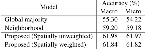
Model Macro MicroAccuracy (%) Global majority 55.30 54.22
Neighborhood 59.20 59.18
[image:6.595.180.417.64.145.2]Proposed (Spatially unweighted) 61.98 61.97 Proposed (Spatially weighted) 61.84 61.82
Table 1: Results of missing value imputation.
we derive the modified log-likelihood function
L(θ, λ, β; xobs) = log ∑
x′
lat
P(xobs⊕x′lat|θ, λ, β). (2)
We perform gradient-based training to maximize the objective. A simple gradient ascent algorithm would updateλas follows:
λ←λ+ηt∂L(θ, λ, β; x∂λ obs), (3)
whereηtis a learning rate that decays according to timet. Instead of the simple gradient ascent algorithm,
an adaptive extension of the optimization algorithm called Adam (Kingma and Ba, 2015) is used.θand βare updated similarly.
The derivative of the log-likelihood function with respect toλis ∂L(θ, λ, β; xobs)
∂λ = Ex′lat∼P(x′lat|xobs,θ,λ,β)
[
S(xobs⊕x′lat) ]
−Ex′∼P(x′|θ,λ,β)[S(x′)]. (4)
Both terms are computationally intractable due to the combinatorial explosion in the number of possible statex′. We approximate the expectation with samples. We collect samples ofx′ from the probability distribution and take the average ofS(x′) to estimate the expectation. We use Gibbs sampling to gen-erate samples ofx′. They are obtained by iteratively updatingx′
i, one element of x′ while keeping the
remaining portionx′
−ifixed. The next value ofx′iis stochastically selected according to
P(x′i =k|x′−i, θ, λ, β)∝exp (θgi,k+λhi,k+βk), (5)
wheregi,kis the number ofi’s neighbors in the spatial neighbor graph taking the valuek(or the sum of the
edge weights for the weighted spatial neighbor graph). hi,k is defined analogously for the phylogenetic
neighbor graph. For the first term of Eq. 4, we only updatex′
lat while keeping xobs unchanged. All elements are updated for the second term.
λandθare initialized with 0.βkis set to the log-probability of taking the valuekinxobs. In this initial setting, Eq. 5 reduces to the empirical probability according toxobsand forcesxlatto largely imitatexobs.
5 Experimental Results 5.1 Missing Value Imputation
We indirectly evaluated the model performance with missing value imputation. If neighboring languages have some predictive power, our model must predict missing values better than chance. Although we have no ground truth for the missing portion of the original database, we can evaluate MVI by hiding some observed features and checking how well they were recovered. For each feature type, we conducted 10-fold cross validation.
We used the default settings for the hyperparameters of Adam (Kingma and Ba, 2015) (not to be confused with the parameters of the autologistic model): β1 = 0.9, β2 = 0.999andϵ = 10−8. We ran 100 iterations for parameter estimation. After that, we sampledxlat as follows. After 50 burn-in iterations, we collected 150 consecutive samples, one per iteration. For each language, we chose the most frequent feature value among the collected samples as the final output.
Features 0.0
0.2 0.4 0.6 0.8 1.0
Accur
acy Baseline
[image:7.595.125.475.111.306.2]Proposed
Figure 2: The MVI accuracy of the proposed model compared with that of the neighborhood baseline on a per-feature basis. Each cross denotes the accuracy of the proposed model with respect to a feature while the corresponding baseline accuracy is marked by a circle. Features are ordered in ascending order of the accuracy of the proposed model.
-0.01 0.00 0.01 0.02 0.03 Spatial association θ
0.000 0.025 0.050
Ph
ylogenetic
association
λ
Phonology Morphology
Nominal Categories Verbal Categories Word Order Simple Clause Lexicon
[image:7.595.87.511.471.676.2]Feature type Accuracy (%) 143G Minor morphological means of signaling negation 99.31
11A Front Rounded Vowels 93.99
90C Postnominal relative clauses 93.39
130A Finger and Hand 88.91
18A Absence of Common Consonants 87.34
38A Indefinite Articles 36.23
37A Definite Articles 35.48
1A Consonant Inventories 34.85
144A Position of Negative Word With Respect to Subject, Object, and Verb 28.45 144L The Position of Negative Morphemes in SOV Languages 16.75
(a) Features ranked by MVI accuracy of the proposed model.
Feature type Difference (%)
51A Position of Case Affixes +14.03
90A Order of Relative Clause and Noun +11.31
116A Polar Questions +10.81
3A Consonant-Vowel Ratio +9.25
69A Position of Tense-Aspect Affixes +9.17
26A Prefixing vs. Suffixing in Inflectional Morphology -3.72 144B Position of negative words relative to beginning and end of clauseand with respect to adjacency to verb -4.55 144L The Position of Negative Morphemes in SOV Languages -7.26
4A Voicing in Plosives and Fricatives -7.79
129A Hand and Arm -8.75
[image:8.595.96.512.63.216.2](b) Features ordered by gain or loss. The proposed model is compared with the neighborhood baseline.
Table 2: Top 5 and bottom 5 features selected by two criteria.
Global majority Choose the most frequent value amongxobsand always output the value.
Neighborhood For each language, collect neighbors inxobs and draw a value from the empirical distri-bution. If one of the two graphs has no observed neighbor, choose the other. If both are available, randomly choose one. If neither is available, draw from the empirical distribution according to the wholexobs.
The proposed model itself had two variants: one with the unweighted spatial neighbor graph and the other with the weighted graph.
The results are shown in Tables 1 and 2(a). Our model outperformed the two baselines although the improvement was not so impressive as that of the dependency-based methods (Murawaki, 2015; Takamura et al., 2016). The edge weighting for the spatial neighbor graph had little effect on imputation performance.
Table 2(b) and Figure 2 compare the proposed model (spatially unweighted) with the neighborhood baseline in detail. As observed by Takamura et al. (2016), huge improvements were observed for Feature 81A “Order of Subject, Object and Verb” and some other word order related features. By contrast, the accuracy dropped sharply for Feature 144L “The Position of Negative Morphemes in SOV Languages,” which might be explained by its mosaic-like distribution.
5.2 Parameter Estimation
[image:8.595.88.508.64.410.2]Feature type θ 143G Minor morphological means of signaling negation 0.0330
11A Front Rounded Vowels 0.0233
144A Position of Negative Word With Respect to Subject, Object, and Verb 0.0206
19A Presence of Uncommon Consonants 0.0183
81A Order of Subject, Object and Verb 0.0177
94A Order of Adverbial Subordinator and Clause 0.0031
37A Definite Articles 0.0024
8A Lateral Consonants 0.0020
3A Consonant-Vowel Ratio 0.0011
144L The Position of Negative Morphemes in SOV Languages -0.0120 (a) Features ranked by the spatial associationθ.
Feature type λ
143G Minor morphological means of signaling negation 0.0833
7A Glottalized Consonants 0.0486
90A Order of Relative Clause and Noun 0.0426 90C Postnominal relative clauses 0.0347
87A Order of Adjective and Noun 0.0334
26A Prefixing vs. Suffixing in Inflectional Morphology 0.0016
38A Indefinite Articles -0.0007
69A Position of Tense-Aspect Affixes -0.0033 144L The Position of Negative Morphemes in SOV Languages -0.0043
129A Hand and Arm -0.0059
[image:9.595.105.492.58.397.2](b) Features ranked by the phylogenetic associationλ.
[image:9.595.101.499.64.213.2]Table 3: Features ranked byθandλ. Top 5 and bottom 5 features are shown for each parameter.
Table 3 shows top- and bottom-ranked features for each parameter, and Figure 3 depicts the relations between the two parameters. 43 out of 47 features were in the top-right quadrant, meaning that they were both spatially and phylogenetically predictive. Nearly all word order-related features were given positive λ, which was consistent with previous findings (Daum´e III, 2009). Wichmann and Holman (2009) also judged Feature 38A “Indefinite Articles” as “very unstable” although their result disagree with ours for Feature 69A “Position of Tense-Aspect Affixes” (stable) and Feature 129A “Hand and Arm” (stable).
In this study, we used genera to construct the phylogenetic neighbor graph, and thus λcan be seen as a genus-level global stability index. Although Feature 83A “Order of Object and Verb” is considered phylogenetically stable by the model, it is well known that the OV languages of India and predominantly VO languages of Europe constitute the Indo-European language family. Much work needs to be done to uncover deep phylogenetic relations. Despite the limitation, we argue that our present study presents a first necessary step toward typology-based phylogenetic inference.
6 Conclusion
In this paper, we quantitatively characterized features of linguistic typology with respect to vertical and horizontal transmission. We presented an autologistic model with which we can estimate the relative strength of transmission. Our model is simple and extensible, and the result are easy to interpret because the two modes of transmission are directly contrasted.
Acknowledgments
We thank Mark N. Grote and Mary C. Towner for providing their code. Needless to say, any oversights and mistakes are ours. This work was partly supported by JSPS KAKENHI Grant Number 26730122.
References
Julian Besag. 1974. Spatial interaction and the statistical analysis of lattice systems.Journal of the Royal
Statisti-cal Society. Series B (MethodologiStatisti-cal), pages 192–236.
Remco Bouckaert, Philippe Lemey, Michael Dunn, Simon J. Greenhill, Alexander V. Alekseyenko, Alexei J. Drummond, Russell D. Gray, Marc A. Suchard, and Quentin D. Atkinson. 2012. Mapping the origins and
expansion of the Indo-European language family. Science, 337(6097):957–960.
Lyle Campbell. 2006. Areal linguistics. InEncyclopedia of Language and Linguistics, Second Edition, pages
454–460. Elsevier.
Mark Collard and Stephen J. Shennan. 2000. Ethnogenesis versus phylogenesis in prehistoric culture change: a case-study using European Neolithic pottery and biological phylogenetic techniques. In Colin Renfrew and
Katherine V. Boyle, editors,Archaeogenetics: DNA and the Population Prehistory of Europe. McDonald
Insti-tute for Archaeological Research.
Sara Grac¸a da Silva and Jamshid J Tehrani. 2016. Comparative phylogenetic analyses uncover the ancient roots
of Indo-European folktales.Royal Society Open Science, 3(1).
Hal Daum´e III and Lyle Campbell. 2007. A Bayesian model for discovering typological implications. InACL,
pages 65–72.
Hal Daum´e III. 2009. Non-parametric Bayesian areal linguistics. InHLT-NAACL, pages 593–601.
Dan Dediu and Michael Cysouw. 2013. Some structural aspects of language are more stable than others: A
comparison of seven methods. PLoS ONE, 8(1):1–20.
Dan Dediu. 2010. A Bayesian phylogenetic approach to estimating the stability of linguistic features and the
genetic biasing of tone. Proc. of the Royal Society of London B: Biological Sciences, 278(1704):474–479.
Aharon Dolgopolsky. 1998. The Nostratic Macrofamily and Linguistic Palaeontology. The McDonald Institute
for Archaeological Research.
Michael Dunn, Angela Terrill, Ger Reesink, Robert A. Foley, and Stephen C. Levinson. 2005. Structural
phylo-genetics and the reconstruction of ancient language history. Science, 309(5743):2072–2075.
Michael Dunn, Simon J. Greenhill, Stephen C. Levinson, and Russell D. Gray. 2011. Evolved structure of
language shows lineage-specific trends in word-order universals. Nature, 473(7345):79–82.
Joseph Felsenstein. 1981. Evolutionary trees from DNA sequences: A maximum likelihood approach. Journal of
Molecular Evolution, 17(6):368–376.
Russell D. Gray and Quentin D. Atkinson. 2003. Language-tree divergence times support the Anatolian theory of
Indo-European origin. Nature, 426(6965):435–439.
Joseph H. Greenberg, editor. 1963.Universals of language. MIT Press.
Joseph H. Greenberg. 2000. Indo-European and Its Closest Relatives: The Eurasiatic Language Family, Volume
1: Grammar. Stanford: Stanford University Press.
Simon J. Greenhill, Quentin D. Atkinson, Andrew Meade, and Russel D. Gray. 2010. The shape and tempo of
language evolution. Proc. of the Royal Society B, 277(1693):2443–2450.
Harald Hammarstr¨om, Robert Forkel, Martin Haspelmath, and Sebastian Bank, editors. 2016.Glottolog 2.7. Max
Planck Institute for the Science of Human History.
Martin Haspelmath, Matthew Dryer, David Gil, and Bernard Comrie, editors. 2005. The World Atlas of Language
Structures. Oxford University Press.
Julie Josse, Marie Chavent, Benot Liquet, and Franc¸ois Husson. 2012. Handling missing values with regularized
Diederik Kingma and Jimmy Ba. 2015. Adam: A method for stochastic optimization. In 3rd International Conference for Learning Representations.
M. Paul Lewis, Gary F. Simons, and Charles D. Fennig, editors. 2014. Ethnologue: Languages of the World, 17th
Edition. SIL International. Online version: http://www.ethnologue.com.
Giuseppe Longobardi and Cristina Guardiano. 2009. Evidence for syntax as a signal of historical relatedness. Lingua, 119(11):1679–1706.
Yugo Murawaki. 2015. Continuous space representations of linguistic typology and their application to
phyloge-netic inference. InProc. of NAACL-HLT, pages 324–334.
Shijulal Nelson-Sathi, Johann-Mattis List, Hans Geisler, Heiner Fangerau, Russell D. Gray, William Martin, and
Tal Dagan. 2010. Networks uncover hidden lexical borrowing in Indo-European language evolution.
Proceed-ings of the Royal Society B.
Johanna Nichols. 1992.Linguistic Diversity in Space and Time. University of Chicago Press.
Johanna Nichols. 1994. The apread of language around the Pacific rim. Evolutionary Anthropology: Issues, News,
and Reviews, 3(6):206–215.
Johanna Nichols. 1995. Diachronically stable structural features. In Henning Andersen, editor,Historical
Lin-guistics 1993. Selected Papers from the 11th International Conference on Historical LinLin-guistics, Los Angeles 16–20 August 1993. John Benjamins Publishing Company.
Mark Pagel, Quentin D. Atkinson, Andreea S. Calude, and Andrew Meade. 2013. Ultraconserved words point to
deep language ancestry across Eurasia. Proc. of the National Academy of Sciences, 110(21):8471–8476.
Mikael Parkvall. 2008. Which parts of language are the most stable? STUF-Language Typology and Universals
Sprachtypologie und Universalienforschung, 61(3):234–250.
Thomas Pellard. 2009. ¯Ogami―´El´ements de description d’un parler du Sud des Ry¯uky¯u. Ph.D. thesis, Ecole des
Hautes Etudes en Sciences Sociales (EHESS). (in French).
Morris Swadesh. 1971. The Origin and Diversification of Language. Aldine Atherton.
Hiroya Takamura, Ryo Nagata, and Yoshifumi Kawasaki. 2016. Discriminative analysis of linguistic features for
typological study. InProc. of LREC, pages 69–76.
Yee Whye Teh, Hal Daum´e III, and Daniel Roy. 2008. Bayesian agglomerative clustering with coalescents. In NIPS, pages 1473–1480.
Mary C. Towner, Mark N. Grote, Jay Venti, and Monique Borgerhoff Mulder. 2012. Cultural macroevolution on
neighbor graphs: Vertical and horizontal transmission among western north American Indian societies.Human
Nature, 23(3):283–305.
Nikolai Sergeevich Trubetzkoy. 1928. Proposition 16. InActs of the First International Congress of Linguists,
pages 17–18.
Tasaku Tsunoda, Sumie Ueda, and Yoshiaki Itoh. 1995. Adpositions in word-order typology. Linguistics,
33(4):741–762.
Søren Wichmann and Eric W. Holman. 2009. Temporal Stability of Linguistic Typological Features. Lincom
Europa.
Søren Wichmann. 2015. Diachronic stability and typology. In Claire Bowern and Bethwyn Evans, editors,The