Combining Linguistic Features with Weighted Bayesian Classifier
for Temporal Reference Processing
Guihong Cao Department of Computing
The Hong Kong Polytechnic University, Hong Kong [email protected]
Wenjie Li Department of Computing
The Hong Kong Polytechnic University, Hong Kong [email protected]
Kam-Fai Wong
Department of Systems Engineering and Engineering Management
The Chinese University of Hong Kong, Hong Kong [email protected]
Chunfa Yuan
Department of Computer Science and Technology Tsinghua University, Beijing, China.
Abstract
Temporal reference is an issue of determining how events relate to one another. Determining temporal relations relies on the combination of the information, which is explicit or implicit in a language. This paper reports a computational model for determining temporal relations in Chinese. The model takes into account the ef-fects of linguistic features, such as tense/aspect, temporal connectives, and discourse structures, and makes use of the fact that events are repre-sented in different temporal structures. A ma-chine learning approach, Weighted Bayesian Classifier, is developed to map their combined effects to the corresponding relations. An em-pirical study is conducted to investigate differ-ent combination methods, including lexical-based, grammatical-lexical-based, and role-based methods. When used in combination, the weights of the features may not be equal. Incor-porating with an optimization algorithm, the weights are fine tuned and the improvement is remarkable.
1 Introduction
Temporal information describes changes and time of the changes. In a language, the time of an event may be specified explicitly, for example “他 们 在
1997年解决了该市的交通问题 (They solved the traf-fic problem of the city in 1997)”; or it may be related to the time of another event, for example “修成立交 桥以后, 他们解决了该市的交通问题 (They solved the traffic problem of the city after the street bridge had
been built”. Temporal reference describes how
events relate to one another, which is essential to natural language processing (NLP). Its major appli-cations cover syntactic structural disambiguation (Brent, 1990), information extraction and question answering (Li, 2002), language generation and ma-chine translation (Dorr, 2002).
Many researchers have attempted to characterize the nature of temporal reference in a discourse. Iden-tifying temporal relations1 between two events
1 The relations under examined include both intra-sentence and
inter-pends on a combination of information resources. This information is provided by explicit tense and aspect markers, implicit event classes or discourse structures. It has been used to explain semantics of temporal expressions (Moens, 1988; Webber, 1988), to constrain possible temporal interpretations (Hitzeman, 1995; Sing, 1997), or to generate appro-priate temporally conjoined clauses (Dorr, 2002).
The purpose of our work is to develop a computa-tional model, which automatically determines tempo-ral relations in Chinese. While tempotempo-ral reference interpretation in English has been well studied, Chi-nese has been rarely discussed. In our study, thirteen related features are identified from linguistic per-spective. How to combine these features and how to map their combined effects to the corresponding rela-tions are the critical issues to be addressed in this paper.
Previous work was limited in that they just con-structed constraint or preference rules for some rep-resentative examples. These methods are ineffective for computing purpose, especially when a large number of the features are involved and the interac-tion among them is unclear. Therefore, a machine learning approach is applied and the empirical stud-ies are carried out in our work.
The rest of this paper is organized as follows. Sec-tion 2 introduces temporal relaSec-tion representaSec-tions. Section 3 provides linguistic background of temporal reference and investigates linguistic features for de-termining temporal relations in Chinese. Section 4 explains the methods used to combine linguistic fea-tures with Bayesian Classifier. It is followed by a description of the optimization algorithm which is used for estimating feature weights in Section 5. Fi-nally, Section 6 concludes the paper.
2 Representing Temporal Relations
With the growing interests to temporal information processing in NLP, a variety of temporal systems have been introduced to accommodate the character-istics of temporal information. In order to process temporal reference in a discourse, a formal
tation of temporal relations is required. Among those who worked on representing or explaining temporal relations, some have taken the work of Reichenbach (Reichenbach, 1947) as a starting point, while others based their works on Allen’s (Allen, 1983).
Reichenbach proposed a point-based temporal the-ory. Reichenbach’s representation associated English tenses and aspects with three time points, namely event time (E), speech time (S) and reference time (R). The reference of E-R and R-S was either before (or after in reverse order) or simultaneous. This the-ory was later enhanced by Bruce who defined seven temporal relations (Bruce, 1972). Given two durative events, the interval relations between them were modeled by the order between the greatest lower bounding point and least upper bounding point of the two events. In the other camp, instead of adopting time points, Allen took intervals as temporal primi-tives to facilitate temporal reasoning and introduced thirteen basic relations. In this interval-based repre-sentation, points were relegated to a subsidiary status as “meeting places” of intervals. An extension to Allen’s theory, which treated both points and inter-vals as primitives on an equal footing, was later in-vestigated by Knight and Ma (Knight, 1994).
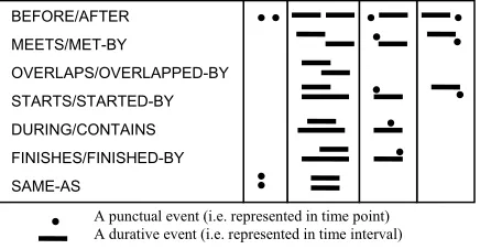
[image:2.595.62.280.573.686.2]In natural languages, events described can be ei-ther punctual or durative in nature. A punctual event, e.g., 爆炸 (explore), occurs instantaneously. It takes time but does not last in a sense that it lacks of a process of change. It is adequate to represent a punc-tual event with a simple point structure. Whilst, a durative event, e.g., 盖楼 (built a house), is more complex and its accomplishment as a whole involves a process spreading in time. Representing a durative event requires an interval representation. For this reason, Knight and Ma’s model is adopted in our work (see Figure 1). Taking the sentence “修成立交 桥以后, 他们解决了该市的交通问题 (They solved the traffic problem of the city after the street bridge had been built)” as an example, the relation held between building the bridge (i.e., an interval) and solving the problem (i.e., a point) is BEFORE.
Figure 1 13 relations represented with points and intervals
3 Linguistic Background of Temporal Refer-ence in a Discourse
3.1 Literature Review
There were a number of theories in the literature about how temporal relations between events can be determined in English. Most of the researches on
temporal reference were based on Reichenbach’s notion of tense/aspect structure, which was known as Basic Tense Structure (BTS). As for relating two events adjoined by a temporal/causal connective, Hornstein (Hornstein, 1990) proposed a neo-Reichenbach structure which organized the BTSs into a Complex Tense Structure (CTS). It has been argued that all sentences containing a matrix and an adjunct clause were subject to linguistic constraints on tense structure regardless of the lexical words in-cluded in the sentence. Generally, constraints were used to support syntactic disambiguation (Brent, 1990) or to generate acceptable sentences (Dorr, 2002).
In a given CTS, a past perfect clause should pre-cede the event described by a simple past clause. However, the order of two events in CTS does not necessarily correspond to the order imposed by the interpretation of the connective (Dorr, 2002). Tem-poral/casual connective, such as “after”, “before” or “because”, can supply explicit information about the temporal ordering of events. Passonneau (Passon-neau, 1988), Brent (Brent, 1990 and Sing (Sing, 1997) determined intra-sentential relations by accounting for temporal or causal connectives. Dorr and Gaast-erland (Dorr, 2002), on the other hand, studied how to generate the sentences which reflect event tempo-ral relations by selecting proper connecting words. However, temporal connectives can be ambiguous. For instance, a“when” clausepermits many possible temporal relations.
Several researchers have developed the models that incorporated aspectual types (such as those dis-tinct from states, processes and events) to interpret temporal relations between clauses connected with “when”. Moens and Steedmen (Moens, 1988) devel-oped a tripartite structure of events2, and emphasized it was the notion of causation and consequence that played a central role in defining temporal relations of events. Webber (Webber, 1988) improved upon the above work by specifying rules for how events are related to one another in a discourse and Sing and Sing defined semantic constraints through which events can be related (Sing, 1997). The importance of aspectual information in retrieving proper aspects and connectives for sentence generation was also recognized by Dorr and Gaasterland (Dorr, 2002).
Some literature claimed that discourse structures suggested temporal relations. Lascarides and Asher (Lascarides, 1991) investigated various contextual effects on rhetorical relations (such as narration, elaboration, explanation, background and result). They corresponded each of the discourse relations to a kind of temporal relation. Later, Hitzeman (Hitze-man, 1995) described a method for analyzing tempo-ral structure of a discourse by taking into account the effects of tense, aspect, temporal adverbials and
2 The structure comprises a culmination, an associated preparatory process and a consequence state.
A punctual event (i.e. represented in time point) A durative event (i.e. represented in time interval)
BEFORE/AFTER MEETS/MET-BY
torical relations. A hierarchy of rhetorical and tempo-ral relations was adopted so that they could mutually constrain each other.
To summarize, the interpretation of temporal rela-tions draws on the combination of various informa-tion resources, including explicit tense/aspect and connectives (temporal or otherwise), temporal classes implicit in events, or rhetorical relations hid-den in a discourse. This conclusion, although drawn from the studies of English, provides the common understanding on what information is required for determining temporal relations across languages. 3.2 Linguistic Features for Determining Tem-poral Relations in Chinese
Thirteen related linguistic features are recognized for determining Chinese temporal relations in this paper (See Table 1). The selected features are scat-tered in various grammatical categories due to the unique nature of language, but they fall into the fol-lowing three groups.
(1) Tense/aspect in English is manifested by verb inflections. But such morphological variations are inapplicable to Chinese verbs. Instead, they are conveyed lexically. In other words, tense and as-pect in Chinese are expressed using a combination of, for example, time words, auxiliaries, temporal position words, adverbs and prepositions, and particular verbs. They are known as Tense/Aspect Markers.
(2) Temporal Connectives in English primarily in-volve conjunctions, such as “after” and “before”, which are the key components in discourse struc-tures. In Chinese, however, conjunctions, conjunc-tive adverbs, prepositions and position words, or their combinations are required to represent connectives. A few verbs that express cause/effect imply a temporal relation. They are also regarded as a feature relating to discourse structure3. The words which contribute to the tense/aspect and temporal connective expressions are explicit in a sentence and generally known as Temporal
3 The casual conjunctions such as “because” are included in this group.
tors.
(3) Event Classes are implicit in a sentence. Events can be classified according to their inherent tem-poral characteristics, such as the degree of telicity and atomicity. The four widespread accepted tem-poral classes are state, process, punctual event and developing event (Li, 2002). Based on their classes, events interact with the tense/aspect of verbs to determine the temporal relations between two events.
Temporal indicators and event classes are both re-ferred to as Linguistic Features. Table 1 shows the association between a temporal indicator and its ef-fects. Note that the association is not one-to-one. For example, adverbs affect tense/aspect (e.g. 正, being) as well as discourse structure (e.g. 边, at the same time). For another example, tense/aspect can be jointly affected by auxiliary words (e.g. 过 ,
were/was), trend verbs (起来, begin to), and so on. Obviously, it is not a simple task to map the com-bined effects of the thirteen linguistic features to the corresponding relations. Therefore, a machine learn-ing approach is proposed, which investigates how these features contribute to the task and how they should be combined.
4 Combining Linguistic Features with Machine Learning Approach
Previous efforts in corpus-based NLP have incor-porated machine learning methods to coordinate mul-tiple linguistic features, for example, in accent resto-ration (Yarowsky, 1994) and event classification (Siegel, 1998).
Temporal relation determination can be modeled as a relation classification task. We formulate the thirteen temporal relations (see Figure 1) as the classes to be decided by a classifier. The classifica-tion process is to assign an event pair to one class according to their linguistic features. There existed numerous classification algorithms based upon su-pervised learning principle. One of the most effective classifiers is Bayesian Classifier, introduced by Duda
and Hart (Duda, 1973) and analyzed in more detail by Langley and Thompson (Langley, 1992). Its pre-dictive performance is competitive with
state-of-the-Linguistic Feature Symbol POS Tag Effect Example
With/Without punctuations PT Not Applicable Not Applicable Not Applicable
Speech verbs VS TI_vs Tense 报告, 表示, 称
Trend verbs TR TI_tr Aspect 起来, 下去
Preposition words P TI_p Discourse Structure/Aspect 当, 到, 继
Position words PS TI_f Discourse Structure 底, 后, 开始
Verbs with verb objects VV TI_vv Tense/Aspect 继续, 进行, 续
Verbs expressing wish/hope VA TI_va Tense 必须, 会, 可
Verbs related to causality VC TI_vc Discourse Structure 导致, 致使, 引起
Conjunctive words C TI_c Discourse Structure 并, 并且, 不过
Auxiliary words U TI_u Aspect 着, 了, 过
Time words T TI_t Tense 过去, 今后, 今年
Adverbs D TI_d Tense/Aspect/Discourse Structure 便, 并, 并未, 不
Event class EC E0/E1/E2/E3 Event Classification State, Punctual Event,
art classifiers, such as C4.5 and SVM (Friedman, 1997).
4.1 Bayesian Classifier
Given the classc, Bayesian Classifier learns from training data the conditional probability of each at-tribute. Classification is performed by applying Bayes rule to compute the posterior probability of c given a particular instancex, and then predicting the class with the highest posterior probability ratio. Let
] ,..., , , ,
[e1 e2 t1 t2 tn
x= , e1,e2∈E are the two event classes and t1,t2,...,tn∈Tare the temporal indicators (i.e. the words). E is the set of event classes. T is the set of temporal indicators. Thenxis classified as:
= ) ,..., , , , | ( ) ,..., , , , | ( log max arg 2 1 2 1 2 1 2 1 * n n
c Pc e e t t t
t t t e e c P c (E1)
where cdenotes the classes different fromc. As-suming event classes are independent of temporal indicators givenc, we have:
= ) ( ) | ,..., , , , ( ) ( ) | ,..., , , , ( log ) ,..., , , , | ( ) ,..., , , , | ( log 2 1 2 1 2 1 2 1 2 1 2 1 2 1 2 1 c P c t t t e e P c P c t t t e e P t t t e e c P t t t e e c P n n n n (E2) + + = ) | ,..., , ( ) | ,..., , ( log ) | , ( ) | , ( log ) ( ) ( log 2 1 2 1 2 1 2 1 c t t t P c t t t P c e e P c e e P c P c P n n
Assuming temporal indicators are independent of each other, we have
∏ = = n i i i n n c t P c t P c t t t P c t t t P 1 2 1 2 1 ) | ( ) | ( ) | ,..., , ( ) | ,..., , (
, (i=1,2,...n) (E3) A Naïve Bayesian Classifier assumes strict inde-pendence among all attributes. However, this as-sumption is not satisfactory in the context of tempo-ral relation determination. For example, if the relation betweene1 and e2 is SAME_AS, e1 and e2
have to be identical. We release the independence assumption fore1ande2, and decompose the second part of (E2) as:
) , | ( ) | ( ) , | ( ) | ( ) | , ( ) | , ( 1 2 1 1 2 1 2 1 2 1 c e e P c e P c e e P c e P c e e P c e e P = (E4)
Estimation of p(e2|e1,c) is motivated by Absolute Discounting N-Gram language model (Goodman, 2001): = > − = 0 ) , , ( if ) | ( ) , ( 0 ) , , ( if ) , ( ) , , ( ) , | ( 1 2 2 1 1 2 1 1 2 1 2 c e e C c e P c e c e e C c e C D c e e C c e Pe α (E5)
hereD is the discount factor and is set to 0.5 experi-mentally. From the fact that ( | , ) 1
2 1 2 = ∑ e c e e
P , we get:
∑ ∑ > > − − = 0 ) , , ( | 2 0 ) , , (
| 2 1
1 1 2 2 1 2 2 ) | ( 1 ) , | ( 1 ) , ( c e e C e c e e C e c e P c e e P c e α (E6) ) | (t c
p i and p(ei|c) are estimated by MLE with
Dirichlet Smoothing method:
∑ ∈ + + = T t i i i i T u c t C u c t C c t P | | ) , ( ) , ( ) |
( (i=1,2,...n)
(E7) ∑ ∈ + + = E e i i i i E u c e C u c e C c e P | | ) , ( ) , ( ) |
( (i=1,2)
(E8) where u (=0.5) is the smoothing factor. Then,
) | (t c
p i , p(ei|c)and P(e2|e1,c) can be estimated
with (E5) - (E8) by substituting c with c.
4.2 Estimating P(t1,t2,...tn|c) with Lexical-POS Information
The effects of a temporal indicator are constrained by its positions in a sentence. For instance, the con-junctive word 因为 (because) may represent the dif-ferent relations when it occurs before or after the first event. Therefore, in estimating p(t1,t2,...tn|c), we consider an indicator located in three positions: (1) BEFORE the first event; (2) AFTER the first event and BEFORE the second and it modifies the first event; (3) the same as (2) but it modifies the second event; and (4) AFTER the second event. Note that cases (2) and (3) are ambiguous. The positions of the temporal indicators are the same. But it is uncertain whether these indicators modify the first or the sec-ond event if there is no punctuation (such as comma, period, exclamation or question mark) separating their roles. The ambiguity is resolved by using POS information. We assume that an indicator modifies the first event if it is an auxiliary word, a trend word or a position word; otherwise it modifies the second.
Thus, we rewrite P(t1,t2,...tn|c) as P(t11,...,t1n1,
) | ,... , ,..., ,
,..., 2 2 31 33 41 4 4 21 t t t t t c
t n n n , wherenjis the total
number of the temporal indicators occurring in the position j . j=1,2,3,4 represents the four positions and n n
j j =
∑
= 4 1. Assumingtjiare independent of each
other, then
∏
= n i i c t P 1 ) |
( in (E3) is revised as
∏ ∏
= = 4 1 1 ) | ( j n i ji j c tP . Accordingly, (E7) is revised as:
∑ ∈ + + = T t ji ji ji ji T u c t C u c t C c t P | | ) , ( ) , ( ) | (
(j=1,2,3,4 and i=1,2,...nj)
(E7’)
In addition to taking positions into account, we further classify the temporal indicators into two groups according to their grammatical categories or semantic roles. The rationale of grouping will be demonstrated in Section 4.3.
4.3 Experimental Results
partitioned equally into two sets. One is similar as training data in class distribution, while the other is quite different. 209 lexical words, gathered from lin-guistic books and corpus, are used as the temporal indicators and manually marked with the tags given in Table 1.
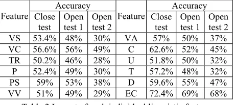
4.3.1 Impact of Individual Features
From linguistic perspective, the thirteen features (see Table 1) are useful for temporal relation deter-mination. To examine the impact of each individual feature, we feed a single linguistic feature to the Bayesian Classifier learning algorithm one at a time and study the accuracy of the resultant classifier. The experimental results are given in Table 2. It shows that event classes have greatest accuracy, followed by conjunctions in the second place, and adverbs in the third in the close test. Since punctuation shows no contribution, we only use it as a syntactic feature to differentiate cases (2) and (3) mentioned in Sec-tion 4.2.
4.3.2 Features in Combination
We now use Bayesian Classifier introduced in Sec-tions 4.1 and 4.2 to combine all the related temporal indicators and event classes, since none of the fea-tures can achieve a good result alone. The simplest way is to combine the features without distinction. The conditional probabilityP(tji|c)is estimated by (E7’). This model is called Ungrouped Model (UG).
However, as illustrated in table 1, the temporal in-dicators play different roles in building temporal ref-erence. It is not reasonable to treat them equally. We claim that the temporal indicators have two functions, i.e., representing the connections of the clauses, or representing the tense/aspect of the events. We iden-tify them as connective words or tense/aspect mark-ers and separate them into two groups. This allows features to be compared with those in the same group. Let T =[T1,T2], where T1is the set of connective
words and T2is the set of tense/aspect markers. We
have 1 1 1
2 1
1,t ,..,t T
t m∈ andt12,t22,..,tl2∈T2 , mand l are the number of the connective words and the tense/aspect markers in a sentence respectively. We assume that the occurrences of the two groups are independent. By taking both grouping and position features into account, we replace
∏
= n
i i
c t P
1
) |
( with
∏∏∏
= = =
2
1 4
1 1
) | (
k j
n
i k ji
k j
c t
P ,k=1,2 represents the two groups
and j
k k
j n
n =
∑
=
2
1
. To build the grouping-based Bayes-ian Classifier, (E7’) is modified as:
∑
∈ +
+ =
k k ji T
t
k k
ji k ji k
ji
T u c t C
u c t C c
t P
| | ) , (
) , ( )
| (
(k=1,2, j=1,2,3,4 and i=1,2,...nj)
(E7’’)
4.3.3 Grouping Features by Grammatical Cate-gories or Semantic Roles
We partition temporal indicators into connective words and tense/aspect markers in two ways. One is simply based on their grammatical categories (i.e. POS information). It separates conjunctions (e.g., 然 后, after; 因为, because) and verbs relating to causal-ity (e.g., 导致, cause) from others. They are assumed to be connective words (i.e.∈T1), while others are
tense/aspect markers (i.e.∈T2). This model is called
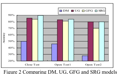
Grammatical Function based Grouping Model (GFG). Unfortunately, such a separation is ineffective. In comparison with UG, the performance of GFG de-creases as shown in figure 2. This reveals the com-plexity of Chinese in connecting expressions. It arises from the fact that some other words, such as adverbs (e.g., 边…边, meanwhile), prepositions (e.g., 在, at) and position words (e.g., 之前, before), can also serve such a connecting function (see Table 1). Actually, the roles of the words falling into these grammatical categories are ambiguous. For instance, the adverb才can express an event happened in the past, e.g., “他才刚刚写完报告 (He just finished the report)”. It can be also used in a connecting expres-sion (such as 才…又…), e.g., “他才写完报告又去图 书馆了(He went to the library after he had finished the report)”.
This finding suggests that temporal indicators should be divided into two groups according to their semantic roles rather than grammatical categories. Therefore we propose the third model, namely Semantic Role based Grouping Model (SRG), in which the indicators are manually re-marked as TI_j_pos or TI_at_pos4.
Figure 2 shows the accuracies of four models (i.e. DM. UG, GFG and SRG) based on the three tests. Test 1 is the close test carried out on training data and tests 2 and 3 are open tests performed on differ-ent test data. DM (i.e., Default Model) assigns all incoming cases with the most likely class and it is used as evaluation baseline. In our case, it is SAME_AS, which holds 50.2% in training data. SRG model outperforms UG and GFG models. These results validate our previous assumption em-pirically.
4 “j” and “at” are the tags representing connecting and tense/aspect roles respectively. “pos” is the POS tag of the temporal indicator TI. Accuracy Accuracy
Feature Close test
Open test 1
Open test 2
Feature Close test
Open test 1
Open test 2
VS 53.4% 48% 30% VA 57% 50% 37%
VC 56.6% 56% 49% C 62.6% 52% 45%
TR 50.2% 46% 28% U 51.8% 50% 32%
P 52.4% 49% 30% T 57.2% 48% 32%
PS 59% 53% 38% D 59.6% 55% 47%
[image:5.595.56.286.309.412.2]VV 51% 49% 29% EC 72.4% 69% 68%
20% 30% 40% 50% 60% 70% 80% 90%
Close T est Open T est1 Open T est2
Ac
cu
ra
cy
DM UG GFG SRG
Figure 2 Comparing DM, UG, GFG and SRG models
4.3.4 Impact of Semantic Roles in SRG Model When the temporal indicators are classified into two groups based on their semantic roles in SRG model, there are three types of linguistic features used in the Bayesian Classifier, i.e., tense/aspect markers, connective words and event classes. A set of experiments are conducted to investigate the im-pacts of each individual feature type and the imim-pacts when they are used in combination (shown in Table 3). We find that the performance of methods 1 and 2 in the open tests drops dramatically compared with those in the close test. But the predictive strength of event classes in method 3 is surprisingly high. Two conclusions are thus drawn. Firstly, the models using tense/aspect markers and connective words are more likely to encounter over-fitting problem with insuffi-cient training data. Secondly, different features have varied weights. We then incorporate an optimization approach to adjust the weights of the three types of features, and propose an algorithm to tackle over-fitting problem in the next section.
Method Semantic Groups Close test Open test 1 Open test 2
1 Tense/aspect markers 71% 58% 40%
2 Connective words 75% 65% 57%
3 Event classes 66.6% 69% 68%
4 1+2 84.8% 70% 56%
5 1+3 76.6% 72% 66%
6 2+3 82.4% 84% 81%
7 1+2+3 89.8% 84% 80%
[image:6.595.67.266.53.179.2]8 Default 50.2% 46% 28%
Table 3: Impact of Semantic Role based Groups
5. Weighted Bayesian Classifier
Letλ1,λ2,λ3be the weights of event classes,
con-nective words and tense/aspect markers respectively. Then the Weighted Bayesian Classifier is:
) ,..., , , , | (
) ,..., , , , | ( log
2 1 2 1
2 1 2 1
n n
t t t e e c P
t t t e e c P
+ =
) | , (
) | , ( log )
( ) ( log
2 1
2 1
1 P e e c
c e e P c
P c
P λ (E9)
+
+
) | ,..., , (
) | ,..., , ( log )
| ,..., , (
) | ,..., , (
log 2 2
2 2 1
2 2 2 2 1 3
1 1 2 1 1
1 1 2 1 1 2
c t t t P
c t t t P c
t t t P
c t t t P
l l
m m λ
λ
In order to estimate the weights, we need a suit-able optimization approach to search for the opti-mal value of [λ1,λ2,λ3] automatically.
5.1 Estimating Weights with Simulated Anneal-ing Algorithm
Quite a lot optimization approaches are available to compute the optimal value of [λ1,λ2,λ3]. Here, Simulated Annealing algorithm is employed to per-form the task, which is a general and powerful opti-mization approach with excellent global convergence (Kirkpatrick, 1983). Figure 3 shows the procedure of searching for an optimal weight vector with the algo-rithm.
1. k=1, tk =T(tk−1)
2. Generates a random change from the current weight vec-torvi. The updated weight vector is denoted byvj. Then
computes the increasement of the objective function, i.e.
) ( ) (vj f vi
f −
=
∆ .
3 Acceptsvjas an optimal vector and substitutesviwith the following accept rate:
∆
∆ ∆
→ = exp( ) if ><0
0 if 1 ) (
k j
i
t v
v P
4 Ifk<Lk, letsk=k+1, goes to step 2.
5 Else iftk <Tf, goes to step 1.
6 Else stops looping and outputs the current optimal weight vector.
Figure 3 Simulated Annealing algorithm
In Figure 3, Markov chain lengthLk =20; tem-perature update functionT(t)=0.9*t; starting point
] , ,
[ 0
3 0 2 0 1 0 = λ λ λ
v =[1,1,1]; initial temperature t0=20 and final temperature =10−8
f
t . Note that the initial temperature is critical for a simulated annealing algo-rithm (Kirkpatrick, 1983). Its value should assure that the initial accept rate is greater than 90%.
5.2 K-fold Cross-Validation
The accuracy of the classifier is defined as the ob-jective function of the Simulated Annealing algo-rithm illustrated in Figure 3. If it is evaluated with the accuracy over all training data, the Weighted Bayesian Classifier may trap into over-fitting prob-lem and lower the performance due to insufficient data. To avoid this, we employ K-fold Cross-Validation technique. It partitions the original set of data into K parts. One part is selected arbitrarily as evaluating data and the other K-1 parts as training data. Then K accuracies on evaluating data are ob-tained after K iterations and their average is used as the objective function.
[image:6.595.312.535.131.359.2]5.3 Experimental Results
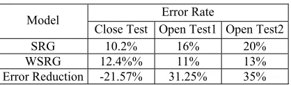
Table 4 shows the result of the experiment which compares WSRG (Weighted SRG) with SRG. We use error reduction to evaluate the benefit from in-corporating weight parameters into Bayesian Classi-fier. It is defined as:
SRG
WSRG SRG
rate error
rate error rate
error
_ _ _
reduction
[image:6.595.64.281.446.565.2]The experimental results show that the Weighted Bayesian Classifier outperforms the Bayesian Classi-fier significantly in the two open tests and it tackles the over-fitting problem well. To test Simulated An-nealing algorithm’s global convergence, we ran-domly choose several initial values and they finally converge to a small area [7.2±0.09, 5.8±0.02, 3.0±0.02]. The empirical result demonstrates that the output of a Simulated Annealing algorithm is a global optimal weighting vector.
6 Conclusions
Temporal reference processing has received grow-ing attentions in last decades. However this topic has not been well studied in Chinese. In this paper, we proposed a method to determine temporal relations in Chinese by employing linguistic knowledge and ma-chine learning approaches. Thirteen related linguistic features were recognized and temporal indicators were further grouped with respect to grammatical functions or semantic roles. This allows features to be compared with those in the same group. To ac-commodate the fact that the different types of fea-tures support varied importance, we extended Naïve Bayesian Classifier to Weighted Bayesian Classifier and applied Simulated Annealing algorithm to opti-mize weight parameters. To avoid over-fitting prob-lem, K-fold Cross-Validation technique was incorpo-rated to evaluate the objective function of the optimi-zation algorithm. Establishing the temporal relations between two events could be extended to provide a determination of the temporal relations among multi-ple events in a discourse. With such an extension, this temporal analysis approach could be incorpo-rated into various NLP applications, such as question answering and machine translation.
Acknowledgements
The work presented in this paper is partially sup-ported by Research Grants Council of Hong Kong (RGC reference number PolyU5085/02E) and CUHK Strategic Grant (account number 4410001).
References
Allen J., 1983. Maintaining Knowledge about Temporal Intervals. Communications of the ACM, 26(11):832-843.
Brent M., 1990. A Simplified Theory of Tense Repre-sentations and Constraints on Their Composition, In Proceedings of the 28th Annual Conference of the
As-sociation for Computational Linguistics, pages 119-126. Pittsburgh.
Bruce B., 1972. A Model for Temporal References and
its Application in Question-Answering Program. Arti-ficial Intelligence, 3(1):1-25.
Dorr B. and Gaasterland T., 2002. Constraints on the Generation of Tense, Aspect, and Connecting Words from Temporal Expressions. submitted to Journal of Artificial Intelligence Research.
Duda, R. O. and P. E. Hart, 1973. Pattern Classification and Scene Analysis. New York.
Friedman N., Geiger D. and Goldszmidt M., 1997. Bayesian Network Classifiers. Machine Learning 29:131-163, Kluwer Academic Publisher.
Goodman J., 2001. A Bit of Progress in Language Mod-eling. Microsoft Research Technical Report MSR-TR-2001-72.
Hitzeman J., Moens M. and Grover C., 1995. Algo-rithms for Analyzing the Temporal Structure of Dis-course. In Proceedings of the 7th European Meeting of the Association for Computational Linguistics, pages 253-260. Dublin, Ireland.
Hornstein N., 1990. As Time Goes By. MIT Press, Cam-bridge, MA.
Kirkpatrick, S., Gelatt C.D., and Vecchi M.P., 1983. Optimization by Simulated Annealing. Science, 220(4598): 671-680.
Knight B. and Ma J., 1997. Temporal Management Us-ing Relative Time in Knowledge-based Process Con-trol, Engineering Applications of Artificial Intelli-gence, 10(3):269-280.
Langley, P.W. and Thompson K., 1992. An Analysis of Bayesian Classifiers. In Proceedings of the 10th
Na-tional Conference on Artificial Intelligence, pages 223–228. San Jose, CA.
Lascarides A. and Asher N., 1991. Discourse Relations and Defensible Knowledge. In Proceedings of the 29th
Meeting of the Association for Computational Lin-guistics, pages 55-62. Berkeley, USA.
Li W.J. and Wong K.F., 2002. A Word-based Approach for Modeling and Discovering Temporal Relations Embedded in Chinese Sentences, ACM Transaction on Asian Language Processing, 1(3):173-206. Moens M. and Steedmen M., 1988. Temporal Ontology
and Temporal Reference. Computational Linguistics, 14(2):15-28.
Passonneau R., 1988. A Computational Model of the Semantics of Tense and Aspect. Computational Lin-guistics, 14(2):44-60.
Reichenbach H., 1947. The Elements of Symbolic Logic. The Free Press, New York.
Siegel E.V. and McKeown K.R., 2000. Learning Meth-ods to Combine Linguistic Indicators: Improving As-pectual Classification and Revealing Linguistic In-sights. Computational Linguistics, 26(4):595-627. Singh M. and Singh M., 1997. On the Temporal
Struc-ture of Events. In Proceedings of AAAI-97 Workshop on Spatial and Temporal Reasoning, pages 49-54. Providence, Rhode Island.
Webber B., 1988. Tense as Discourse Anaphor. Compu-tational Linguistics, 14(2):61-73.
Yarowsky D., 1994. Decision Lists for Lexical Ambi-guity Resolution: Application to the Accent Restora-tion in Spanish and French. In Proceeding of the 32nd
Annual Meeting of the Association for Computational Linguistics, pages 88-95. San Francisco, CA.
Error Rate Model
Close Test Open Test1 Open Test2
SRG 10.2% 16% 20%
WSRG 12.4%% 11% 13%
[image:7.595.67.276.63.124.2]Error Reduction -21.57% 31.25% 35%