Learning Task-specific Bilexical Embeddings
Pranava Swaroop Madhyastha Xavier Carreras Ariadna Quattoni
TALP Research Center Universitat Polit`ecnica de Catalunya
Campus Nord UPC, Barcelona
pranava,carreras,[email protected]
Abstract
We present a method that learns bilexical operators over distributional representations of words and leverages supervised data for a linguistic relation. The learning algorithm exploits low-rank bilinear forms and induces low-dimensional embeddings of the lexical space tailored for the target linguistic relation. An advantage of imposing low-rank constraints is that prediction is expressed as the inner-product between low-dimensional embeddings, which can have great computational benefits. In experiments with multiple linguistic bilexical relations we show that our method effectively learns using embeddings of a few dimensions.
1 Introduction
We address the task of learning functions that compute compatibility scores between pairs of lexical items under some linguistic relation. We refer to these functions as bilexical operators. As an instance of this problem, consider learning a model that predicts the probability that an adjective modifies a noun in a sentence. In this case, we would like the bilexical operator to capture the fact that some adjectives are more compatible with some nouns than others. For example, a bilexical operator should predict that the adjectiveelectronichas high probability of modifying the noundevicebut little probability of modifying the nouncase.
Bilexical operators can be useful for multiple NLP applications. For example, they can be used to reduce ambiguity in a parsing task. Consider the following sentence extracted from a weblog: Vynil can be applied to electronic devices and cases, wooden doors and furniture and walls. If we want to predict the dependency structure of this sentence we need to make several decisions. In particular, the parser would need to decide (1) Doeselectronicmodifydevices? (2) Doeselectronicmodifycases? (3) Doeswoodenmodifydoors? (4) Doeswoodenmodifyfurniture? Now imagine that in the corpus used to train the parser none of these nouns have been observed, then it is unlikely that these attachments can be resolved correctly. However, if an accurate noun-adjective bilexical operator were available most of the uncertainty could be resolved. This is because a good bilinear operator would give high probability to the pairselectronic-device,wooden-door,wooden-furnitureand low probability to the pairelectronic-case.
The simplest way of inducing a bilexical operator is to learn it from a training corpus. That is, assuming that we are given some data annotated with a linguistic relation between a modifier and a head (e.g. adjective and noun) we can simply build a maximum likelihood estimator forPr(m|h)by counting the occurrences of modifiers and heads under the target relation. For example, we could consider learning bilexical operators from sentences annotated with dependency structures. Clearly, this model can not generalize to head words not present in the training data.
To mitigate this we could consider bilexical operators that can exploit lexical embeddings, such as a distributional vector-space representation of words. In this case, we assume that for every word we can compute ann-dimensional vector space representationφ(w) → Rn. This representation typically
captures distributional features of the context in which the lexical item can occur. The key point is that This work is licenced under a Creative Commons Attribution 4.0 International License. Page numbers and proceedings footer are added by the organizers. License details:http://creativecommons.org/licenses/by/4.0/
we do not need a supervised corpus to compute the representation. All we need is a large textual corpus to compute the relevant statistics. Once we have the representation we can exploit operations in the induced vector space to define lexical compatibility operators. For example we could define a bilexical operator as:
Pr(m|h) = Pexp{hφ(m), φ(h)i}
m0exp{hφ(m0), φ(h)i} (1)
wherehφ(x), φ(y)idenotes the inner-product. Alternatively, given an initial high-dimensional distribu-tional representation computed from a large textual corpus we could first induce a projection to a lower kdimensional space by performing truncated singular value decomposition. The idea is that the lower dimensional representation will be more efficient and it will better capture the relevant dimensions of the distributional representation. The bilexical operator would then take the form of:
Pr(m|h) = Pexp{hUφ(m), Uφ(h)i}
m0exp{hUφ(m0), Uφ(h)i} (2)
whereU ∈Rk×nis the projection matrix obtained via SVD. The advantage of this approach is that as
long as we can estimate the distribution of contexts of words we can compute the value of the bilexical operator. However, this approach has a clear limitation: to design a bilinear operator for a target linguistic relation we must design the appropriate distributional representation. Moreover, there is no clear way of exploiting a supervised training corpus.
In this paper we combine both the supervised and distributional approaches and present a learning algorithm for inducing bilexical operators from a combination of supervised and unsupervised training data. The main idea is to define bilexical operators using bilinear forms over distributional representa-tions: φ(x)>W φ(y), whereW ∈Rn×nis a matrix of parameters. We can then train our model on the
supervised training corpus via conditional maximum-likelihood estimation. To induce a low-dimensional representation, we first observe that the implicit dimensionality of the bilinear form is given by the rank ofW. In practice controlling the rank ofW can result in important computational savings in cases where one evaluates a target wordxagainst a large number of candidate wordsy: this is because we can project the representationsφ(x)andφ(y) down to the low-dimensional space where evaluating the function is simply an inner-product. This setting is in fact usual, for example for lexical retrieval applications (e.g. given a noun, sort all adjectives in the vocabulary according to their compatibility), or for parsing (where one typically evaluates the compatibility between all pairs of words in a sentence).
Consequently with these ideas, we propose to regularize the maximum-likelihood estimation using a nuclear norm regularizer that serves as a convex relaxation to the rank function. To minimize the regularized objective we make use of an efficient iterative proximal method that involves computing the gradient of the function and performing singular value decompositions.
We test the proposed algorithm on several linguistic relations and show that it can predict modifiers for unknown words more accurately than the unsupervised approach. Furthermore, we compare different types of regularizers for the bilexical operatorW, and observe that indeed the low-rank regularizer results in the most efficient technique at prediction time.
In summary, the main contributions of this paper are:
• We propose a supervised framework for learning bilexical operators over distributional representa-tions, based on learning bilinear formsW.
• We show that we can obtain low-dimensional compressions of the distributional representation by imposing low-rank constraints to the bilinear form. Combined with supervision, this results in lexical embeddings tailored for a specific bilexical task.
2 Bilinear Models for Bilexical Predictions 2.1 Definitions
LetV be a vocabulary, and letx∈ Vdenote a word. LetH ⊆ Vbe a set of head words, andM ⊆ Vbe a set of modifier words. In the noun-adjective relation example,His the set of nouns andMis the set of adjectives.
The task is as follows. We are given a training set of ltuples D = {(m, h)1, . . . ,(m, h)l}, where
m ∈ Mandh ∈ H and we want to learn a model of the conditional distributionPr(m |h). We want this model to perform well on all head-modifier pairs. In particular we will test the performance of the model on heads that do not appear inD.
We assume that we are given access to a distributional representation function φ : V → Rn, where
φ(x)is then-dimensional representation ofx. Typically, this function is computed from an unsupervised corpus. We useφ(x)[i]to refer to thei-th coordinate of the vector.
2.2 Bilinear Model
Our model makes use of the bilinear form W : Rn×Rn → R, whereW ∈ Rn×n, and evaluates as
φ(m)>W φ(h). We define the bilexical operator as:
Pr(m|h) = exp
φ(m)>W φ(h) P
m0∈Mexp{φ(m0)>W φ(h)} (3)
Note that the above model is nothing more than a conditional log-linear model defined over n2 fea-tures fi,j(m, h) = φ(m)[i]φ(h)[j] (this can be seen clearly when we write the bilinear form as
Pn
i=1Pnj=1fi,j(m, h)Wi,j. The reason why it is useful to regardW as a matrix will become evident in
the next section.
Before moving to the next section, let us note that the unsupervised SVD model in Eq. (2) is also a bilinear model as defined here. This can be seen if we setW =UU>, which is a bilinear form of rank
k. The key difference is in the wayW is learned using supervision.
3 Learning Low-rank Bilexical Operators 3.1 Low-rank Optimization
Given a training setDand a feature functionφ(x)we can do standard conditional max-likelihood opti-mization and minimize the negative of the log-likelihood function,log Pr(D):
X
(m,h)∈D
φ(m)>W φ(h)−log X m0∈M
expnφ(m0)>W φ(h)o (4)
We would like to control the complexity of the learned model by including some regularization penalty. Moreover, like in the dimensional unsupervised approach we want our model to induce a low-dimensional representation of the lexical space. The first observation is that the bilinear form computes a weighted inner product in some space. Consider the singular value decomposition: W = UΣV. We can write the bilinear form as:[φ(m)>U] Σ [V φ(h)], thus we can regardm˜ =φ(m)>U as a projection
ofmand˜h=V φ(h)as a projection ofh. Then the bilinear form can be written as:Pni=1Σ[i,i]m˜[i]˜h[i]. The rank ofW defines the dimensionality of the induced space. It is easy to see that ifW has rankkit can be factorized asUΣV whereU ∈Rn×kandV ∈Rk×n.
Since the rank ofW determines the dimensionality of the induced space, it would be reasonable to add a rank minimization penalty in the objective in (4). Unfortunately this would lead to a non-convex regularized objective. Instead, we propose to use as a regularizer a convex relaxation of the rank function, the nuclear normkWk∗ (the`1 norm of the singular values ofW). Putting it all together, our learning
algorithm minimizes: X
(m,h)∈D
Hereλis a constant that controls the trade-off between fitting the data and the complexity of the model. This objective is clearly convex since both the objective and the regularizer are convex. To minimize it we use the a proximal gradient algorithm which is described next.
3.2 A Proximal Algorithm for Bilexical Operators
We now describe the learning algorithm that we use to induce the bilexical operators from training data. We are interested in minimizing the objective (5), or in fact a more general version where we can replace the regularizerkWk∗by standard`1or`2 penalties. For any convex regularizerr(W)(namely`1,`2 or the nuclear norm) the objective in (5) is convex. Our learning algorithm is based on a simple optimization scheme known asforward-backward splitting (FOBOS)(Duchi and Singer, 2009).
This algorithm has convergence rates in the order of 1/2, which we found sufficiently fast for our application. Many other optimization approaches are possible, for example one could express the regu-larizer as a convex constraint and utilize a projected gradient method which has a similar convergence rate. Proximal methods are slightly more simple to implement and we chose the proximal approach.
The FOBOS algorithm works as follows. In a series of iterations t = 1. . . T compute parameter matricesWtas follows:
1. Compute the gradient of the negative log-likelihood, and update the parameters
Wt+0.5 =Wt−ηtg(Wt)
whereηt= √ct is a step size andg(Wt)is the gradient of the loss atWt.
2. UpdateWt+0.5to take into account the regularization penaltyr(W), by solving
Wt+1 = argmin
W ||Wt+0.5−W||
2
2+ηtλr(W)
For the regularizers we consider, this step is solved using theproximal operatorassociated with the regularizer. Specifically:
• For`1it is a simple thresholding:
Wt+1(i, j) = sign(Wt+0.5(i, j))·max(Wt+0.5(i, j)−ηtλ,0)
• For`2it is a simple scaling:
Wt+1= 1 +1η
tλWt+0.5
• For nuclear-norm, perform SVD thresholding. Compute the SVD to writeWt+0.5 = USV> withSa diagonal matrix andU, V orthogonal matrices. Denote byσi thei-th element on the
diagonal ofS. Define a new matrixS¯with diagonal elementsσ¯i = max(σi−ηtλ,0). Then
set
Wt+1=USV¯ >
4 Related Work
Research in learning representations for natural language processing can be broadly classified into two different paradigms based on the learning setting: unsupervised representation learning and semi-supervised representation learning. Unsemi-supervised representation learning does not require any semi-supervised training data, while semi-supervised representation learning requires the presence of supervised training data with the potential advantage that it can adapt the representation to the task at hand.
Unsupervised approaches to learning representations mainly involve representations that are learned not for a specific task, rather a variety of tasks. These representations rely more on the property of abstractness and generalization. Further, unsupervised approaches can be roughly categorized into (a) clustering-based approaches that make use of clusters induced using a notion of distributed similarity, such as the method by Brown et al. (1992); (b) neural-network-based representations that focus on learn-ing multilayer neural network in a way to extract features from the data (Morin and Bengio, 2005; Mnih and Hinton, 2007; Bengio and S´en´ecal, 2008; Mnih and Hinton, 2009); (c) pure distributional approaches that principally follow the distributional assumption that the words which share a set of contexts are sim-ilar (Sahlgren, 2006; Turney and Pantel, 2010; Dumais et al., 1988; Landauer et al., 1998; Lund et al., 1995; V¨ayrynen et al., 2007).
We also induce lexical embeddings, but in our case we employ supervision. That is, we follow a semi-supervised paradigm for learning representations. Semi-supervised approaches initially learn rep-resentations typically in an unsupervised setting and then induce a representation that is jointly learned for the task with a labeled corpus. A high-dimensional representation is extracted from unlabeled data, while the supervised step compresses the representation to be low-dimensional in a way that favors the the task at hand.
Collobert and Weston (2008) present a neural network language model, where given a sentence, it performs a set of language processing tasks (from part of speech tagging, chunking, extracting named entity, extracting semantic roles and decisions on the correctness of the sentence) by using the learned representations. The representation itself is extracted from unlabeled corpora, while all the other tasks are jointly trained on labeled corpus.
Socher et al. (2011) present a model based on recursive neural networks that learns vector space rep-resentations for words, multi-word phrases and sentences. Given a sentence with its syntactic structure, their model assings vector representations to each of the lexical tokens of the sentence, and then traverses the syntactic tree bottom-up, such that at each node a vector representation of the corresponding phrase is obtained by composing the vectors associated with the children.
Bai et al. (2010) use a technique similar to ours, using bilinear forms with low-rank constraints. In their case, they explicitly look for a low-rank factorization of the matrix, making their optimization non-convex. As far as we know, ours is the first convex formulation, where we employ a relaxation of the rank (i.e. the nuclear norm) to make the objective convex. They apply the method to document ranking, and thus optimize a max-margin ranking loss. In our application to bilexical models, we perform conditional max-likelihood estimation. Hutchinson et al. (2013) propose an explicitly sparse and low-rank maximum-entropy language model. The sparse plus low low-rank setting is learned in such a way that the low rank component learns the regularities in the training data and the sparse component learns the exceptions like multiword expressions etc.
Chechik et al. (2010) also learned bilinear operators using max-margin techniques, with pairwise similarity as supervision, but they did not consider low-rank constraints.
One related area where bilinear operators are used to induce embeddings is distance metric learning. Weinberger and Saul (2009) used large-margin nearest neighbor methods to learn a non-sparse embed-ding, but these are computationally intensive and might not be suitable for large-scale tasks in NLP.
5 Experiments on Syntactic Relations
50 55 60 65 70 75 80 85 90
1e3 1e4 1e5 1e6 1e7 1e8
pairwise accuracy
number of operations Adjectives given Noun
unsupervised NN L1
L2 66
68 70 72 74 76 78 80
1e3 1e4 1e5 1e6 1e7 1e8
pairwise accuracy
number of operations Nouns given Adjective
unsupervised NN L1 L2 46 48 50 52 54 56 58 60 62
1e3 1e4 1e5 1e6 1e7 1e8
pairwise accuracy
number of operations Objects given Verb
unsupervised NN L1 L2 60 65 70 75 80
1e3 1e4 1e5 1e6 1e7 1e8
pairwise accuracy
number of operations Verbs given Object
[image:6.595.78.522.60.505.2]unsupervised NN L1 L2
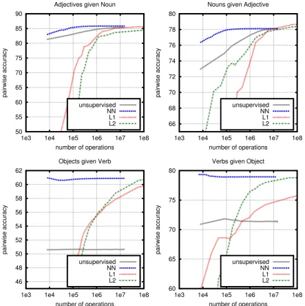
Figure 1: Pairwise accuracy with respect to the number of double operations required to compute the distribution over modifiers for a head word. Plots for noun-adjective and verb-object relations, in both directions.
• Noun-Adjective: we model the distribution of adjectives given a noun; and a separate distribution of nouns given an adjective.
• Verb-Object: we model the distribution of object nouns given a verb; and a separate distribution of verbs given an object.
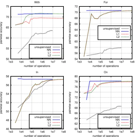
• Prepositions: in this case we consider bilexical operators associated with a preposition, which model the probability of a head noun or verb above the prepositiongiventhe noun below the preposition. We present results for prepositional relations given by “with”, “for”, “in” and “on”.
50 55 60 65 70 75
1e3 1e4 1e5 1e6 1e7 1e8
pairwise accuracy
number of operations With unsupervised NN L1 L2 54 56 58 60 62 64 66 68 70 72
1e3 1e4 1e5 1e6 1e7 1e8
pairwise accuracy
number of operations For unsupervised NN L1 L2 46 48 50 52 54 56 58
1e3 1e4 1e5 1e6 1e7 1e8
pairwise accuracy
number of operations In unsupervised NN L1 L2 60 62 64 66 68 70 72 74 76 78 80
1e3 1e4 1e5 1e6 1e7 1e8
pairwise accuracy
number of operations On
[image:7.595.81.520.59.506.2]unsupervised NN L1 L2
Figure 2: Pairwise accuracy with respect to the number of double operations required to compute the distribution over modifiers for a head word. Plots for four prepositional relations: with, for, in, on. The distributions are of verbs and objects above the preposition given the noun below the preposition.
To test the performance of our algorithm for each relation we partition the set of heads into a training and a test set, 60% of the heads are use for training, 10% of the heads are used for validation and 30% of the heads are used for testing. Then, we consider all observed modifiers in the data to form a vocabulary of modifier words. The goal of this task is to learn conditional distribution over all these modifers given a head word without context. In our experiments, the number of modifiers per relation ranges from 2,500 to 7,500 words. For each head word, we create a list ofcompatiblemodifiers from the annotated data, by taking all modifiers that occur at least once with the head. Hence, for each head the set of all modifiers is partitioned into compatible and non-compatible. For testing, we measure apairwise accuracy, the percentage of compatible/non-compatible pairs of modifiers where the former obtains higher probability. Let us stress that none of the test head words has been observed in training, while the list of modifiers is the same for training, validation and testing.
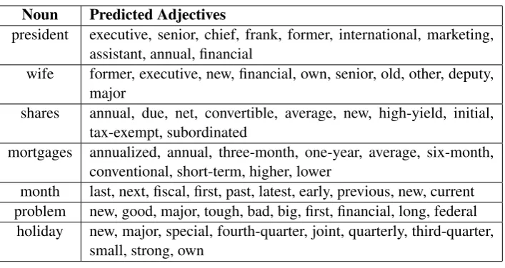
Noun Predicted Adjectives
president executive, senior, chief, frank, former, international, marketing, assistant, annual, financial
wife former, executive, new, financial, own, senior, old, other, deputy, major
shares annual, due, net, convertible, average, new, high-yield, initial, tax-exempt, subordinated
mortgages annualized, annual, three-month, one-year, average, six-month, conventional, short-term, higher, lower
month last, next, fiscal, first, past, latest, early, previous, new, current problem new, good, major, tough, bad, big, first, financial, long, federal
[image:8.595.123.477.59.247.2]holiday new, major, special, fourth-quarter, joint, quarterly, third-quarter, small, strong, own
Table 1: 10 most likely adjectives for some test nouns.
unsupervised model: a low-dimensional SVD model as in Eq. (2), which corresponds to an inner product as in Eq. (1) when all dimensions are considered.
To report performance, we measure pairwise accuracy with respect to the capacity of the model in terms of number of active parameters. To measure the capacity of a model we consider the number of double operations that are needed to compute, given a head, the scores for all modifiers in the vocabulary (we exclude the exponentiations and normalization needed to compute the distribution of modifiers given a head, since this is a constant cost for all the models we compare, and is not needed if we only want to rank modifiers). Recall that the dimension ofφ(x)isn, and assume that there aremtotal modifiers in the vocabulary. In our experimentsn= 2,000andmranges from2,500to7,500. The correspondances with operations are:
• Assume that the L1 and L2 models haveknon-zero weights inW. Then the number of operations to compute a distribution iskm.
• Assume that the NN and the unsupervised models have rankk. We assume that the modifier vectors are alredy projected down tokdimensions. For a new head, one needs to project it and performm inner products, hence the number of operations iskn+km.
Figure 1 shows the performance of models for noun-adjective and verb-object relations, while Figure 2 shows plots for prepositional relations.1 The first observation is that supervised approaches outperform
the unsupervised approach. In cases such as noun-adjetive relations the unsupervised approach performs close to the supervised approaches, suggesting that the pure distributional approach can sometimes work. But in most relations the improvement obtained by using supervision is very large. When comparing the type of regularizer, we see that if the capacity of the model is unrestricted (right part of the curves), all models tend to perform similarly. However, when restricting the size, the nuclear-norm model performs much better. Roughly, 20 hidden dimensions are enough to obtain the most accurate performances (which result in∼140,000operations for initial representaions of2,000dimensions and5,000modifier candidates). As an example of the type of predictions, Table 1 shows the most likely adjectives for some test nouns.
6 Experiments on PP Attachment
We now switch to a standard classification task, prepositional phrase attachment, that we frame as a bilexical prediction task. We start from the formulation of the task as a binary classification problem by Ratnaparkhi et al. (1994): given a tuplex=hv, o, p, niconsisting of a verbv, noun objecto, preposition
55 60 65 70 75 80
for from with
attachment accuracy
[image:9.595.165.438.61.257.2]bilinear L1 bilinear L2 bilinear NN linear interpolated L1 interpolated L2 interpolated NN
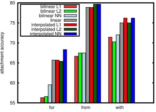
Figure 3: Attachment accuracies of linear, bilinear and interpolated models for three prepositions.
pand nounn, decide if the prepositional phrasep-nattaches tov(y=V) or too(y=O). For example, inhmeet,demand,for,productsithe correct attachment isO.
Ratnaparkhi et al. (1994) define a linear maximum likelihood model of the form
Pr(y|x) = exp{hw, f(x, y)i} ∗Z(x)−1, where f(x, y) is a vector of d features, w is a parame-ter vector in Rd, and Z(x) is the normalizer summing over y = {V,O}. Here we define a bilexical
model of the form that uses a distributional representationφ:
Pr(V|hv, o, p, ni) = exp{φ(v)>W p Vφ(n)}
Z(x) Pr(O|hv, o, p, ni) =
exp{φ(o)>Wp Oφ(n)}
Z(x) (6)
The bilinear model is parameterized by two matricesWVandWOper preposition, each of which captures
the compatibility between nouns below a certain preposition and heads ofVorOprepositional relations, respectively. AgainZ(x)is the normalizer summing overy ={V,O}, but now using the bilinear form. It is straighforward to modify the learning algorithm in Section 3 such that the loss is a negative log-likelihood for binary classification, and the regularizer considers the sum of norms of the model matrices. We ran experiments using the data by Ratnaparkhi et al. (1994). We trained separate models for different prepositions, focusing on the prepositions that are more ambiguous: for, from, with. We compare to a linear “maxent” model following Ratnaparkhi et al. (1994) that uses the same feature set. Figure 3 shows the test results for the linear model, and bilinear models trained with L1, L2, NN regularization penalties. The results of the bilinear models are significantly below the accuracy of the linear model, suggesting that some of the non-lexical features of the linear model (such as prior weighting of the two classes) might be difficult to capture by the bilinear model over lexical representations. To check if the bilinear model might complement the linear model or just be worse than it, we tested simple combinations based on linear interpolations. For a constantλ∈[0,1]we define:
Pr(y|x) =λPrL(y|x) + (1−λ) PrB(y|x) . (7)
We search for the best λon the validation set, and report results of combining the linear model with each of the three bilinear models. Results are shown also in Figure 3. Interpolation models improve over linear models, though only the improvement forforis significant (2.6%). Future work should exploit finer combinations between standard linear features and distributional bilinear forms.
7 Conclusions
learning algorithm induces a low-dimensional representation of the lexical space by imposing low-rank constraints on the parameters of the bilinear form. By means of supervision, our model induces two low-dimensional lexical embeddings, one on each side of the bilexical linguistic relation, and compu-tations can be expressed as an inner-product between the two embeddings. This factorized form of the model can have great computational advantages: in many applications one needs to evaluate the function multiple times for a fixed set of lexical items, for example in dependency parsing. Hence, one can first project the lexical items to their embeddings, and then compute all pairwise scores as inner-products. In experiments, we have shown that the embeddings we obtain in a number of linguistic relations can be modeled with a few hidden dimensions.
As future work, we would like to apply the low-rank approach to other model forms that can employ lexical embeddings, specially when supervision is available. For example, dependency parsing models, or models of predicate-argument structures representing semantic roles, exploit bilexical relations. In these applications, being able to generalize to wordpairsthat are not observed during training is essential. We would also like to study how to combine low-rank bilexical operators, which in essence induce a task-specific representation of words, with other forms of features that capture class or contextual information. One desires that such combinations can preserve the computational advantages behind low-rank embeddings.
Acknowledgements
We thank the reviewers for their helpful comments. This work was supported by projects XLike (FP7-288342), ERA-Net CHISTERA VISEN and TACARDI (TIN2012-38523-C02-00). Xavier Carreras was supported by the Ram´on y Cajal program of the Spanish Government (RYC-2008-02223).
References
Bing Bai, Jason Weston, David Grangier, Ronan Collobert, Kunihiko Sadamasa, Yanjun Qi, Olivier Chapelle, and Kilian Weinberger. 2010. Learning to rank with (a lot of) word features. Information Retrieval, 13(3):291–314, June.
Yoshua Bengio and Jean-S´ebastien S´en´ecal. 2008. Adaptive importance sampling to accelerate training of a neural
probabilistic language model. IEEE Transactions on Neural Networks, 19(4):713–722.
Peter F. Brown, Peter V. deSouza, Robert L. Mercer, Vincent J. Della Pietra, and Jenifer C. Lai. 1992. Class-based
n-gram models of natural language. Computational Linguistics, 18:467–479.
Eugene Charniak, Don Blaheta, Niyu Ge, Keith Hall, and Mark Johnson. 2000. BLLIP 1987–89 WSJ Corpus Release 1, LDC No. LDC2000T43. Linguistic Data Consortium.
Gal Chechik, Varun Sharma, Uri Shalit, and Samy Bengio. 2010. Large scale online learning of image similarity
through ranking.Journal of Machine Learning Research, pages 1109–1135.
Ronan Collobert and Jason Weston. 2008. A unified architecture for natural language processing: Deep neural
networks with multitask learning. InProceedings of the 25th International Conference on Machine Learning,
ICML ’08, pages 160–167, New York, NY, USA. ACM.
John Duchi and Yoram Singer. 2009. Efficient online and batch learning using forward backward splitting.Journal of Machine Learning Research, 10:2899–2934.
Susan T. Dumais, George W. Furnas, Thomas K. Landauer, Scott Deerwester, and Richard Harshman. 1988. Using
latent semantic analysis to improve access to textual information. InSIGCHI Conference on Human Factors in
Computing Systems, pages 281–285. ACM.
Brian Hutchinson, Mari Ostendorf, and Maryam Fazel. 2013. Exceptions in language as learned by the
multi-factor sparse plus low-rank language model. InICASSP, pages 8580–8584.
Thomas K. Landauer, Peter W. Foltz, and Darrell Laham. 1998. An introduction to latent semantic analysis.
Discourse Processes, 25:259–284.
Kevin Lund, Curt Burgess, and Ruth A. Atchley. 1995. Semantic and associative priming in high-dimensional
Mitchell P. Marcus, Beatrice Santorini, and Mary A. Marcinkiewicz. 1993. Building a Large Annotated Corpus of
English: The Penn Treebank.Computational Linguistics, 19(2):313–330.
Andriy Mnih and Geoffrey E. Hinton. 2007. Three new graphical models for statistical language modelling. In
Proceedings of the 24th International Conference on Machine Learning, pages 641–648.
Andriy Mnih and Geoffrey E. Hinton. 2009. A scalable hierarchical distributed language model. InAdvances in
Neural Information Processing Systems, pages 1081–1088.
Frederic Morin and Yoshua Bengio. 2005. Hierarchical probabilistic neural network language model. In
AIS-TATS05, pages 246–252.
Adwait Ratnaparkhi, Jeff Reynar, and Salim Roukos. 1994. A maximum entropy model for prepositional phrase
attachment. In Proceedings of the workshop on Human Language Technology, HLT ’94, pages 250–255,
Stroudsburg, PA, USA. Association for Computational Linguistics.
Magnus Sahlgren. 2006. The Word-Space Model: Using distributional analysis to represent syntagmatic and
paradigmatic relations between words in high-dimensional vector spaces. Ph.D. thesis, Stockholm University. Richard Socher, Jeffrey Pennington, Eric H Huang, Andrew Y Ng, and Christopher D Manning. 2011.
Semi-supervised recursive autoencoders for predicting sentiment distributions. InProceedings of the Conference on Empirical Methods in Natural Language Processing, pages 151–161. Association for Computational Linguis-tics.
Peter D. Turney and Patrick Pantel. 2010. From frequency to meaning: Vector space models of semantics.Journal
of Artificial Intelligence Research, 37(1):141–188, January.
Jaakko J. V¨ayrynen, Timo Honkela, and Lasse Lindqvist. 2007. Towards explicit semantic features using
indepen-dent component analysis. InProceedings of the Workshop Semantic Content Acquisition and Representation
(SCAR), Stockholm, Sweden. Swedish Institute of Computer Science. SICS Technical Report T2007-06. Kilian Q. Weinberger and Lawrence K. Saul. 2009. Distance metric learning for large margin nearest neighbor