Use of an implicit filtering algorithm for mechanical system parameter identification

Title Sheet

COVER INFORMATION FOR SAE TECHNICAL PAPERS

In order to ensure that the correct title, author names, and company affiliations appear on the cover

and title page of your paper, please provide the information requested below.

PAPER TITLE

(upper and lower case):

Use of an Implicit Filtering Algorithm

for Mechanical System Parameter Identification

AUTHORS

COMPANY

(upper and lower case)

(upper and lower case)

1. J. W. David 1. North Carolina State University

2. C.T. Kelley 2. North Carolina State University

ABSTRACT

Optimal design of high-speed valve trains requires the use of an accurate analytical model. While the governing differential equations are important, the coefficients (or parameters) used in these equations are equally as important. Since many of the parameters used in valve train models are difficult to measure directly, parameter identification based on experimental data is required to assure model accuracy.

This paper addresses the parameter identification problem for a valve train model, formulating a scalar cost function which represents the difference in measured and predicted system response. Minimizaton of this cost function yields the 10 unknown system parameters. As the cost function has many local minima, a global optimization scheme must be employed. An implicit filtering algorithm is implemented which applies a scale reduction scheme in conjunction with a gradient projection algorithm to avoid becomming trapped in local minima and thus produces near global minima of the cost function. The implicit filtering algorithm has several tuning parameters which allows its adaptation to many problems. For this problem, implicit filtering proved to be 2 to 4 times more efficient than the adaptive random search method previously employed.

INTRODUCTION

Figure 1 shows a schematic of a typical push-rod type valve train which is the focus of this study. In the design and optimization of such mechanisms for high-speed internal combustion engines, an accurate analytical model is essential. Whether the model is simple [1,2] or complex [3,4], accurate parameters are essential for the accuracy of the model. For linear systems, parameter estimation is a rather mature art while for nonlinear systems the problem of determining system parameters is much more difficult. In that a valve train is a transient mechanism with some components exhibiting steady-state response [5], the problem of parameter estimation is increasingly difficult.

Figure 1: A Typical Pushrod Valve Train [4]

THE MODEL

Figure 2 shows a schematic of a model developed by Kim and David [4] for use in high-speed valve train analysis. It has the advantage of being computationally efficient while having good accuracy for engine speeds of 9,000 rpm and above. This model has several parameters which physically describe the mechanism. The mass parameters can be directly measured and are thus not a problem in this case. The valve spring reactive force, as well parameters k5 and c5, are also easily determined. However, the stiffness parameters k1

through k4 are not easily measured and the damping

Figure 2: Schematic of the Valve Train Model [4]

EXPERIMENTAL APPARATUS AND TEST RESULTS

The test apparatus consists of an engine block less the connecting rods and pistons and with a straight shaft replacing the crankshaft. It has a complete valve train including the cam drive mechanism. A 30 hp direct current motor is used to drive the assembly. Various sensors are used to measure the dynamic response of the mechanism, such as strain-gages, accelerometers, and proximeters. The camshaft rotation angle is measured with an optical encoder which triggers a computer to acquire data.

Figure 3 shows a typical valve motion trace obtained from a short-range proximeter. The valve is initially closed and as it begins to open, the proximeter measures the displacement. Next, the valve moves outside the range of the sensor and thus, the displacement curve is flat. Then, the proximeter senses the valve on the closing event and measures the subsequent displacement. Notice that after closing, the valve bounces off the seat, often more than once. The amplitude of this first bounce is an excellent indicator of the dynamic performance of the mechanism [6] and is used for future comparisons. The range of the proximeter used in this test is about 1.5 mm. Other sensors, such as long range proximeters, are capable of measuring the entire displacement curve of the valve. However, results indicate that the precision of the short range data shown in Figure 3 produces better correlation of the analytical model due to the increased resolution in the valve seating area and subsequent definition of the valve bounce phenomena. Data is taken at a family of engine speeds, usually 7,000 rpm to limiting speed (between 9,000 rpm and 12,000 rpm for the type of valve train presented here) in increments of 100 rpm. Thus, an experiment produces a family of 20 or more displacement curves like Figure 3 that are used in the parameter identification.

- 2 - 1.5 - 1 - 0.5 0 0.5

Ca mshaft A ngle (d eg)

V

al

v

e L

ift

(mm)

0 60 120 180 240 300

Figure 3: Short Range Proximeter Measurement of Valve Motion [5]

COST FUNCTION

Because the system is transient and highly nonlinear, the parameter identification is cast as a least squares error between the predicted response of the model and the experimental data. This error is summed over the number of data points and number of test engine speeds:

f

w y j

j i

y

i

j

j npoints

i nspeed

=

−

=

=

∑

∑

( ( )

*

( ))

2

1 1

(1)

where yj is any predicted system response and yj* is the corresponding measured response. For this study, the response is the valve motion. The weighting function wj is included to exclude the data for which the valve is out of range of the sensor. It can also be used to weight other data points to increase/decrease correlation with a particular portion of the data. The experimental data can be any measurable quantity of the valve train, or even multiple sensor readings (such as proximeter and strain-gage measurements). As the predicted response of the model is a function of the unknown parameters, the goal is to minimize the error between the measured and predicted responses. In an ideal situation with no modeling misconceptions or numerical errors, the cost function would be zero.

THE OPTIMIZATION PROBLEM

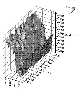
Figures 4 and 5 show three dimensional sections of the optimization landscape. Figure 4 is a plot of the total cost function against two of the unknown parameters and figure 5 is a similar plot with the cost function computed using only a single engine speed.

Figure 4: Cost Function Variation with Two Parameters

Figure 5: Cost Function Variation for Two Parameters, Single RPM

Non-standard optimizers must be used to drive the cost function to a small value. However, one does not need and should not expect to find the global minimum. A sensible goal of an optimization of a function of this kind is simply to find a value of the parameters that make the objective function small. There may be several such sets of values of the parameters and the valve train models based on those sets of parameters will have similar characteristics.

In this paper, implicit filtering [7] performs a sequence of optimizations with varying resolution, thereby seeking to capture the low-frequency behavior of the objective and find a low function value without becoming trapped in a local minimum before reaching an acceptable parameter set.

THE OPTIMIZER: IMPLICIT FILTERING

Implicit filtering, originally proposed in the context of computer aided design of semiconductors [8,9,10] is a generalization of the gradient projection algorithm of [11] in which derivatives are computed with difference quotients. The step sizes (called scales) in the difference quotients are changed as the iteration progresses with the goal of avoiding local minima that are caused by high-frequency, low amplitude oscillations such as those seen in Figs. 4 and 5. Real filtering could be performed, but this requires sampling and filtering the entire solution space and thus, is computationally quite expensive. Implicit filtering is very similar to adaptive meshing schemes used by the computational fluid mechanics community to avoid unwanted harmonics. The algorithm is fully described in [7] and [12]. A brief summary is presented here.

Gradient projection algorithms are variations of the steepest descent method. The goal is to solve the constrained optimization problem

min ( )

x∈ΩΩ

f

x

(2)

where x is the vector of unknown parameters to be determined. The feasible set of solutions

Ω

is defined by simple bounds

{

}

Ω

Ω =

x l

i

≤ ≤

x

i

u

i . (3)

Here xi is the ith component of the vector x. Central to the gradient projection algorithm is the ease with which a vector

x can be projected onto ΩΩ. The projection of P onto ΩΩ is

defined by

P ( )

i

i i i

i i i

i i i i

x

l

x

l

u

x

u

x

l

x

u

=

≤

≥

<

<









if

if

if

(4)

where li is the ith component of the vector representing lower bounds on the solution and ui is the ith component of the vector representing upper bounds on the solution. The gradient projection iteration from a current approximation xc to a better approximation x+ is defined by

x

₊

=

P x

(

_c

−

a

∇

∇

f(

x

_c

)

)

(5) where α is a step length parameter determined so that ƒ(x+) is smaller than ƒ(xc).

If the gradients are approximated by finite differences, ∇ƒ∇ is

replaced by some difference approximation ∇∇hƒ where

∇

∇hƒ could be forward, backward, or centered differences. In

(

∇

_h

( ))

=

(

+

h

)

−

(

−

h

)

h

f

_i

f

i

f

i

x

x

e

x

e

2

(6)

where ei is the ith canonical basis vector. For such an approximation, accuracy of the order of h2 is expected. The convergence theory of Gilmore and Kelley [13] applies to both centered and one sided differences. Experience in using this algorithm in semiconductor applications indicates that centered differences work far better and thus are used in this work.

The iterative scheme involves calculating the gradient using Equation 6. This is then used in Equation 3 and 4 to determine a candidate solution x+. This candidate solution x+ is then checked for sufficient descent by

f

c

f

c

(

x

)

−

(

x

₊

)

≥

σ

x

−

x

+

α

2

(7)

If Equation 7 is satisfied, the candidate solution x+ is accepted and the iteration continues by repeating the above steps up to a limiting value kmax times. If Equation 7 is not satisfied, α is reduced as

α βα

=

(8)

,with 0<

β

<1, a new candidate solution x+ is calculated from eqs. 3 and 4 and checked using Equation 7. This is repeated up to jmax times until an acceptable solution x+ is found. If an acceptable solution is not found in this process, is usually means that the step size h (or scale) is too large and needs to be reduced. This is done in the implicit filtering algorithm.

The iteration is terminated whenever

x

₊

−

x

_c

≤

τ

h

(9)

is below a desired tolerance.

The adaptation of the gradient projection algorithm to implicit filtering is rather simple. Successive applications of the gradient search algorithm are performed using ever decreasing scales. This is done a total of m times. This has the effect of filtering out higher harmonics of the cost function in the early stages of the iteration while admitting them in the final stages of the iteration to improve final convergence. Once the convergence criteria (7) is satisfied for all scales, the algorithm is restarted using the best-to-date solution and rechecked to assure convergence for all scales.

COMPUTATIONAL RESULTS

The implementation of implicit filtering is contained in a code named IFFCO. IFFCO can be obtained by anonymous ftp to math.ncsu.edu in the directory pub\kelley\iffco. Users are advised to get both the FORTRAN code iffco.f and the users’ guide ug.ps. The inputs to the code are:

1. the objective function ƒ 2. the initial guess of the solution 3. the bounds {ui} and {li}

4. an estimate ƒscale for the minimum absolute value of ƒ

5. τ, the constant used in the termination criteria

6. maximum number of step size reductions m

7. the maximum number of step length reductions jmax 8. the maximum number of iterates for each use of the

gradient projection algorithm kmax

Of these, ƒscale , τ, m, jmax and kmax are parameters that the user can tune to improve the performance of IFFCO.

The bounds on the variables are scaled, using {ui} and {li}, to

be between 0 and 1. The function f is divided by ƒscale in order to make the estimated maximum value of f approximately 1. These two scalings are intended to assist the gradient projection algorithm avoid terminations on the initial iteration or after too many step length reductions. The algorithm appears to be relatively insensitive to ƒscale and using the function value from the initial guess is reasonable.

τ reflects the estimate of the amplitude of the high frequency noise in the problem. If the amplitude of τ is small and the noise amplitude is large, the convergence criteria (eq. 7) might never be satisfied. Small amplitude noise would require a small value of τ. If τ is too large, the convergence criteria will be satisfied too easily causing the scale to be reduced too soon, admitting high frequency components into the cost function evaluation. This will cause IFFCO to become trapped in a local minimum. Thus, this is the most important parameter and must be determined by experimentation with each problem undertaken. For this problem, τ=0.1 worked well.

Since the problem is now bounded by 0 and 1, the scale (step size) h per application of the gradient projection algorithm is defined as h=2-i. Other variations are possible, but this one worked well for this problem. The number of step reductions

m should be large enough to provide good resolution of the

solution. For this problem m = 10 was used.

The maximum number of iterates kmax and jmax are tuned to allow the iterative schemes to proceed long enough for successful termination without being so large as to use excessive computational effort. For this problem 5 was used for both.

solutions, given enough time. Thus, one must look at computational efficiency to assess the superior technique.

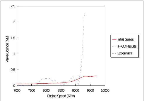
7000 7500 8000 8500 9000 9500 10000

0 0.5 1 1.5 2 2.5

Engine Speed (RPM)

V al ve B ou nc e (M M ) Initial Guess IFFCO Results Experiment

Figure 6: Experimental Results, Initial Guess and IFFCO Results

Figure 7 shows the results of a comparison between IFFCO and the adaptive random search (ARS) technique. Upper bounds and lower bounds are the same for both techniques and z represents the distance between the upper and lower bounds used for the initial guess; i.e.

x

_i

= +

l

_i

(

u

_i

−

l z

_i

)

(10)

For both methods, iteration was stopped when the cost function reached the same goal. In all cases, IFFCO obtained solutions in 1/3 to 1/4 of the number of iterations as ARS.

0 100 200 300 AAAA AAAA AAAA AAAA AAAA AAAA AAAA AAAA AAAA AAAA AAAA AAAA AAAA AAAA AAAA AAAA AAAA AAAA AAAA AAAA AAAA AAAA AAAA AAAA AAAA AAAA AAAA AAAA AAAA AAAA AAAA AAAA AAAA AAAA AAAA AAAA AAAA AAAA AAAA AAAA AAAA AAAA AAAA AAAA AAAA AAAA AAAA AAAA AAAA AAAA AAAA AAAA AAAA AAAA AAAA AAAA AAAA AAAA AAAA AAAA AAAA AAAA AAAA AAAA AAAA AAAA AAAA AAAA AAAA AAAA AAAA AAAA AAAA AAAA AAAA AAAA AAAA AAAA AAAA AAAA AAAA AAAA AAAA AAAA AAAA AAAA AAAA AAAA AAAA AAAA AAAA AAAA AAAA AAAA AAAA AAAA AAAA AAAA AAAA AAAA AAAA AAAA AAAA AAAA AAAA AAAA AAAA AAAA AAAA AAAA AAAA AAAA AAAA AAAA AAAA AAAA AAAA AAAA AAAA AAAA AAAA AAAA AAAA AAAA AAAA AAAA AAAA AAAA AAAA AAAA AAAA AAAA AAAA AAAA AAAA AAAA AAAA AAAA AAAA AAAA AAAA AAAA AAAA

Initial Guess Parameter z

F un c tion E v a lu a tio n s

0.01 0.1 0.2 0.4

IFFCO ARS AAAA AAAA

Figure 7: Cost Function Evaluations as a Function of Initial Guess

Figure 8 shows a comparison of cost function evaluations obtained after 60 iterations. In all cases, the solution obtained by IFFCO is half the value obtained by ARS.

0 0.01 0.02 0.03 0.04 AAAA AAAA AAAA AAAA AAAA AAAA AAAA AAAA AAAA AAAA AAAA AAAA AAAA AAAA AAAA AAAA AAAA AAAA AAAA AAAA AAAA AAAA AAAA AAAA AAAA AAAA AAAA AAAA AAAA AAAA AAAA AAAA AAAA AAAA AAAA AAAA AAAA AAAA AAAA AAAA AAAA AAAA AAAA AAAA AAAA AAAA AAAA AAAA AAAA AAAA AAAA AAAA AAAA AAAA AAAA AAAA AAAA AAAA AAAA AAAA AAAA AAAA AAAA AAAA AAAA AAAA AAAA AAAA AAAA AAAA AAAA AAAA AAAA AAAA AAAA AAAA AAAA AAAA AAAA AAAA AAAA AAAA AAAA AAAA AAAA AAAA AAAA AAAA AAAA AAAA AAAA AAAA AAAA AAAA AAAA AAAA AAAA AAAA AAAA AAAA AAAA AAAA AAAA AAAA AAAA AAAA AAAA AAAA AAAA AAAA AAAA AAAA AAAA AAAA AAAA AAAA AAAA AAAA AAAA AAAA AAAA

Initial Guess Parameter z

C os t F un ct io n

0.01 0.1 0.2 0.4

IFFCO ARS

AAAA AAAA AAAA

Figure 8: Cost Function Value as a Function of Initial Guess for 60 Iterations

CONCLUSIONS

Implicit filtering appears to be an efficient method for parameter identification of high-speed, nonlinear valve trains. Reductions of computation effort as high as 75% were realized over the adaptive random search technique. Some numerical experiments are required, however, to adjust the tuning parameters to achieve optimal results.

ACKNOWLEDGMENTS

The authors wish to gratefully acknowledge Mr. Jim Covey of the GM Motorsports Technology Group for his support of the valve train research and the National Science Foundation for their support of the optimization research under grant DMS-9321938.

REFERENCES

[1] P. Barkan, Calculation fof High-Speed Valve Motion with

a Flexible Overhead Linkage, SAE Transactions, Vol. 61,

1953, pp. 687-700

[2] G.I. Johnson, Studying Valve Dynamics with Electronic

Computers, SAE Progress in Technology, Vol. 5, 1963, pp.

10-28.

[3] A.P. Pisano and F. Freudenstein, An Experimental and

Analytical Investigation of the Dynamic Response of a High-Speed Cam Follower System. Part 2: A Combined, Lumped/Distributed Parameter Dynamic Model, ASME

Journal of Mechanisms, Transmissions, and Automation in Design, Vol. 105, Dec. 1983, pp. 699-704.

[4] D. Kim and J.W. David, A Combined Model for

High-Speed Valve Train Dynamics, Partly Linear and Partly Nonlinear, SAE Technical Paper Series 901726.

[5] D. Kim, Dynamics and Optimal Design of High Speed

Valve Train Systems, Ph. D thesis, Mechanical and Aerospace

[6] J.W. David and D. Kim, Optimal Design of High Speed

Valve Train Systems, SAE Paper 942502, 1994 Motor

Sports Conference Proceedings, Vol. 2, Engines and Drivelines, pp. 103-109.

[7] P. Gilmore and C.T. Kelley, An Implicit Filtering

Algorithm for Optimization of Functions with Many Local Minima, SIAM Journal of Optimization, Vol. 5, No. 2, May

1995.

[8] D. Stoneking, G. Bilbro, R. Trew, P. Gilmore and C.T. Kelley, Yield Optimization Using a GaAs Process Simulator

Coupled to a Physical Device Model, Proceedings

IEEE/Cornell Conference on Advanced Concepts in High Speed Devices and Circuits, IEEE, 1991, pp. 374-383

[9] D. Stoneking, G. Bilbro, R. Trew, P. Gilmore and C.T. Kelley, Yield Optimization Using a GaAs Process Simulator

Coupled to a Physical Device Model, IEEE Transactions on

Microwave Theory and Techniques, 40 (1992), pp.

1353-1363.

[10] D. Stoneking, G. Bilbro, R. Trew, P. Gilmore and C.T. Kelley, Simulated Performance Optimization of GaAs

MESFET Amplifiers, Proceedings IEEE/Cornell Conference on Advanced Concepts in High Speed Devices and Circuits, IEEE, 1991, pp. 393-402.

[11] D.B. Bertsekas, On the Goldstein-Levitin-Polyak

Gradient Projection Method, IEEE Transactions on

Automatic Control, 21 (1976), pp. 174-184.

[12] P. Gilmore and C.T. Kelley, , An Implicit Filtering

Algorithm for Optimization of Functions with Many Local Minima, Tech. Report CRSC-TR94-23, North Carolina State

University, Center for Research in Scientific Computation, December, 1994.

[13] C.T. Kelley, Iterative Methods for Linear and Nonlinear

Equations, SIAM Frontiers in Applied Mathematics,

Philadelphia, 1995 (to appear).

[14] A. Liu, System Identification and Optimal Design of

High Speed Valve Train Systems, Ph. D thesis, Mechanical