Volume 8, No. 3, March – April 2017
International Journal of Advanced Research in Computer Science
RESEARCH PAPER
Available Online at www.ijarcs.info
Spatial Classification and Prediction in Hyperspectral Remote Sensing Data using
Random Forest by Tuning Parameters
Nandhini K
Department of Computer Science Bharathiar University
Coimbatore, India
Porkodi R
Department of Computer Science Bharathiar University
Coimbatore, India
Abstract: Over the past decades hyperspectral remote sensing data have been emerging in identifying the geographical patterns and predicting its behaviour. A digital remote sensing data offers, many practices in learning, exploring, monitoring and understanding the behaviour of the earth surfaces. The hyperspectral remote sensing data is an advanced technique where the topological information are collected in spectral with more number of bands. Inculcating the information from the hyperspectral data relies on the data mining approaches where the data contains many spectral bands and huge temporal information. It requires an front running algorithm to yield high accuracy. The random forest technique is one of the best tree based techniques where optimal solutions are captured at high end construction of possible trees. The mission of this research paper is to give detailed analysis of tuning the parameters of random forest technique based on variable importance, conditional inference and quantile forest applied to AVIRIS Indian pine site-3 hyperspectral data to predict the class labels. The experiment result of random forest with variable importance shows high accuracy of 94.93% in predicting the class labels. Conditional inference and quantile forests are also achieved high accuracy with slight difference of 94.65% and 93.46% respectively.
Keywords: Data mining, Hyperspectral data, Remote sensing, Hyperspectral classification, Random forest
I. INTRODUCTION
The hyperspectral (HS) remote sensing data is one of the major advancement in investigating the behaviour and prediction of the topological area. There are diverse applications in domain using HS data are urbanized for Climatology, Astronomy, Oceanography, Agriculture, Defense etc. The HS data are collected from airborne and spaceborne sensors which capture the Earth's surface and it inculcates the information from trajectories of stored data. The hyperspectral sensor is also known as an imaging spectrometer (Anthony Gualtieri et.al, 2009) [1] used widely for many different application such as Bioinformatics, Insurance, Natural disaster Management etc. Sensor data contains the information of spectral, temporal and geographical resolution of our earth platforms (José M. Bioucas-Dias, et.al, 2013)[2]. Hyperspectral (HS) data generates a hundreds of narrow bands [3], where the dimensionality is crucial which combats the data scientist with it requirement of high computing environment and performance. The issues related with space and time which includes spatial points (Latitude and Longitude) and temporal (time-oriented) information are also known spatio-temporal. The way of collecting data through remote sensing involves active or passive remote sensors. Visual, Optical, Infrared, microwave, RADAR, Satellite and Airborne are different remote sensing types which has been used widely in different applications. Quality of remote sensing data is based on the spatial, radiometric, spectral solution and temporal information. Recent decades of high evolving remote sensing technology shows the major contribution in Hyperspectral data analysis, in which data are collected through airborne or space borne and it covers the huge land areas [4]. Hyperspectral data presents the detailed information of every pixel and it will collect hundreds of narrow spectral bands concurrently.
HS data contains high spectral resolutions and more number of bands, increases the computation complexity and dimensionality. Moreover, these data contains the temporal
information where the time series of the topological pattern analysis have been taken place to vision the future consequences. The curse of dimensionality and accuracy in prediction has been handled with utmost care by the data mining classification techniques. The classification models use the two different learning approaches such as supervised learning and semi supervised learning which emphasize on training and testing the class labels. SVM, Random Forest, Linear models, Neural network models, etc., are some of the classification models, used diversely in many applications and resulted high accuracy in HS classification and Prediction.
The Section I discusses about the introduction of hyperspectral data and broad view about the involvement of data mining classification. Section II gives a detailed analysis of remote sensing data classification with the infer of the spatial and temporal data mining techniques and Section III briefly discuss about the methods used in the random forests and its background. The results and discussion are explained in Section IV and Section V concludes this research work.
.
II. LITERATURE REVIEW
Sequence Mining algorithm) [3]. GSP and Prefix span works on horizontal databases and SPADE works on Vertical databases. Mining topological patterns from a spatio-temporal database by candidate generation and test methodology is not scalable in case of huge patterns. For mining Star-like, Clique and Star-Clique are topological patterns and their geographical features are identified using time window threshold, distance threshold, spatio-temporal and geographical feature database are the basic components for formulation for identifying relationship of distance to geographical features.(Hsu et.al, 2008) [16]. There are most frequent data mining functionalities are widely used to understand the attributes and accuracy in prediction. Apriori algorithm with two dimensional Association analysis, Triangular Kernel Nearest Neighbour algorithm, K –means with Euclidean distance, Support Vector Regression, PCA, Gaussian Mixture Model(GMM) and Markov Random Field (MRF) are combined or used individually for predicting spatio-temporal data and enables decision making [17].
A. Inference of Data mining Techniques in HS Classification
The prospect of the data mining, always high in playing a vital role in hyperspectral image classification which exhibits the information depends on the user needs and appropriate techniques will be applied for accuracy. Some of learning techniques often uses to increase the support of the classification accuracy, especially in hyperspectral remote sensing data and its prediction. The machine learning techniques have been evolved with many subsets such as Deep learning, Active Learning and Extreme Learning. This chapter shows the contribution of above learning techniques with the remote sensing hyperspectral data.
Symbolic and statistical are the two different approaches which come under Machine learning. Also these learning tasks are fall under the following categories, they are Supervised Learning, Unsupervised Learning and Semi supervised learning. The above categories are widely uses many learning methods such as Decision tree, Random forest, linear models etc., in many data mining applications. In supervised learning technique, there are two different approaches such as parametric and non parametric are taken place. The techniques in Parametric approaches are Bayes classifier, Maximum Likelihood, Minimum A - Posterori and minimum risk etc. In nonparametric approach, density estimation and discriminative classification tools are two broad categories. K-Nearest Neighbor (KNN), Kernel estimation, histogram methods and likewise similar techniques are used to estimate the density. Artificial Neural networks (ANN), decision trees, Support vector machines(SVM) are fall under the discriminative classification tools. In the unsupervised classification clustering techniques and mixture models are used to analyze and describe the pattern. SVM, KNN and ANN consumes more time and computational cost are very high (L. Naidoo et.al.,2012)[18].
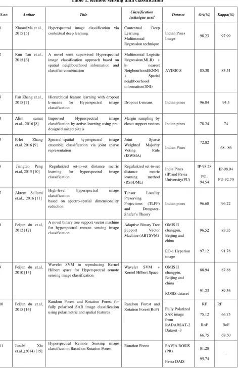
. The Table.1 shows the comparative analysis of classification techniques, dataset used and accuracy achieved for remote sensing data so far. SVM and Random Forest are often applied and most frequently used datasets are Indian pines and ROSIS are widely used to research. Random forest is one of the ensemble learning technique which often used to classify and predict the LIDAR,
multispectral and HS data and it yields high accuracy (V.F. Rodriguez-Galiano,2011)[19]. The classification techniques are necessary to improvise the predicting and analyzing the results in Hyperspectral image. The machine learning and statistical techniques are used widely in HS data.
III. RANDOM FOREST CLASSIFICATION TECHNIQUES
This RF method is a robust when compared to other regression methods which aggregate the decision trees to improve the accuracy. Variable importance and PCA methods are involved to predict the Grassland LAI remote sensed data with Random forest technique (LI Zhen-wang, 2017)[20]. Peiju Du et.al ,2012 [12] applied two integrated approaches of SVM and RF and proposed Distance – weighted dynamic classifier selection (DWDCS) to improve the classification accuracy. The fully polarized SAR image from PolSAR image is classified using RF and Rotation Forest. From the experiment analysis, identified that Random forest technique is comparatively faster than the Rotation forest and SVM (Peiju Du et.al, 2015)[14]. Bolin fu et.al., 2016 [21] compared the random forest algorithm for the HS data by classifying object based and pixel based methods for wetland vegetation mapping using GF1 and SAR data; states that object based classification of RF improves the accuracy. RF model is a reproducible which can be extended over the circumstances and the accuracy performance (Meiling Liu et.al,2014) [22]
S.no. Author Title Classification
technique used Dataset OA(%) Kappa(%)
1 XiaoruiMa et.al., 2015 [5]
Hyperspectral image classification via contextual deep learning
Contextual Deep
A novel semi supervised Hyperspectral image classification approach based on spatial neighbourhood information and classifier combination
Hierarchical feature learning with dropout k-means for Hyperspectral image classification
Dropout k-means Indian pines 96.04 94.5
4 Alim samat
et.al., 2016 [8]
Improved Hyperspectral image classification by active learning using pre-designed mixed pixels
Margin sampling by
closet support vectors Indian pines 78.24 74
5 Erlei Zhang
et.al. 2016 [9]
Spectral–spatial hyperspectral image ensemble classification via joint sparse representation
Regularized set-to-set distance metric learning for hyperspectral image classification
High-level hyperspectral image classification
based on spectro-spatial dimensionality reduction
A novel binary tree support vector machine for hyperspectral remote sensing image classification
Adaptive Binary Tree Support Vector
Wavelet SVM in reproducing Kernel Hilbert space for Hyperspectral remote sensing image classification
Wavelet SVM + Kernel Hilbert Space
OMIS II
Random Forest and Rotation Forest for fully polarized SAR image classification using polarimetric and spatial features
Random Forest and
Rotation Forest(RoF) Fully Polarized SAR image
Hyperspectral Remote Sensing image
classification Based on Rotation Forest Rotation Forest PAVIA ROSIS (PR)
Pavia DAIS
81.28
95.74
The steps involved in the Briemen’s Random Forest are the following,
Algorithm: Briemen’s random forest
Input: Dataset to train : DTn
1. Check the condition tree T value has {1,2….n} then | where n= {1,2,….n}, Number of Trees : T | T>0, nodesize and mtry Output: Prediction of RF at x
do process from step 2 or skip to step 14 2. In training dataset DTn
points a
uniformly select the sample
n
3. Initialize P=( X) holds the list of the cell associated with / without substitute
with the root of the tree
4. Create Pfinal = | empty list { } and initialize A be
the first element of P 5. While P then do
6. Check if the nodesize points are greater than A or equal
7. If it is greater then remove the cell A from the list P 8. Then Concatenate (Pfinal, A). P
9. Else without substitute select uniformly a subset
final
mtry
10. Choose the best cut in A by optimizing the CART split criteria and mtry possible directions
11. Stored the cuts as Aleft and Aright
from the list P
and delete the A
12. Then concatenate (P, Aleft, Aright
13. Calculate the predicted value at x )
14. Calculate the random forest estimation at x if the trees Tn
IV. RESULTS AND DISCUSSION
<0.
This research explored three existing methods of random forest to predict the HS data by stressing on three different factors such as Variable importance, conditional inference and quantile RF. The Fig1 shows the flow of the HS data prediction; train the data by randomly choose the band with minimum class and followed to train the data in RF Variable importance, Conditional inference and Quantile and this model will be tested and evaluated. The RF model parameters are tuned to gain accuracy which was applicable in all three models.
Random forest is the non-parametric tree approach which is the other option of multiple regression. The random forest is measured and predicted using the variable importance and conditional importance. The method involves in both can classification and binary partitioning. INPUT {HS data}
Train the data
Randomly choose the bands with minimal class
Variable Importance
Conditional
Inference Random forest Quantile Random Forest
Tune the parameters mtry, nodesize and M
Predict the HS data using different band less labeled classifiers
Evaluation
Predict Predict
Predict
The random forest technique, basically involved with the below steps for both variable importance and conditional importance respectively. Initially, this method tests the independent variables Ij (I1, I2, I3…… In) , conditional
Inference trees Cj (C1, C2…..Cn) and quantile forest Qj
(Q1,Q2,….Qn) which are strongly associated with the target
variable T and it will choose as per that for the binary split. This will divide the datasets into divide the dataset into two subsets S1 and S2. If any of the subsets have more value, then subset S3 are created. The above steps will be repeated until no longer independent variables Ij, conditional values
Cj and quantile forest Qj
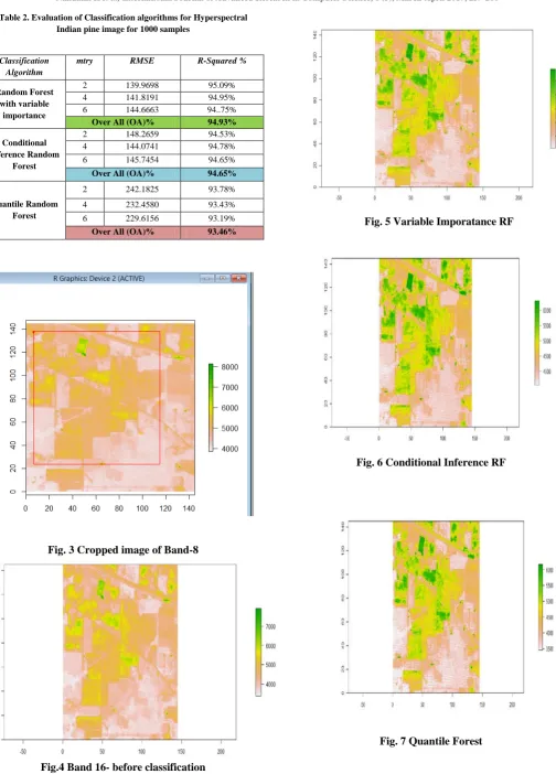
The hyperspectral Indian pines Site 3 image consists of 3 dimensions which are huge and complex in nature. Considering the above difficulties the Band 8 layer has taken and in which extent is cropped and converted as a dataframe for training purpose. But still there are 145 X 145 cell values present in the 220 Bands. So, the subset of 1000 samples are generated for training and tested this model using B16 layer. The Fig. 3 shows the cropped image for training.
After the image has been cropped B 16 layer taken for the testing. The Fig.8 shows the ground reference image which contains many class labels such as Alfalfa, corn-notill, corn-min, corn, Grass/ Pasture, Grass/ Trees etc. The Fig 4 shows the Band 16 contains less class labels. The Fig 5, 6 and 7 shows the predicted results of the variable importance RF, Conditional Inference RF, and Quantile RF.
In this research work there are 6 predictors such as Band 1 to 6 are used for three models with 1000 samples. There are many class labels such as corn, Grass/pasture, wheat, soyabean-clean, building grass – Tree Drives and soybeans-notill are classified perfectly with small samples and predictors.
are not associated with the T respectively [24].
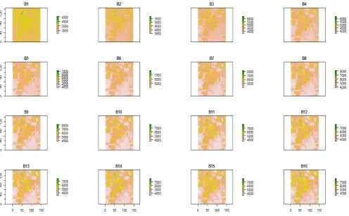
In this research work, Indian pine site 3 dataset have been downloaded from the Purdue University website [25] as a tif file format. The HS data contains three dimensions 145 X 145 X 220 which are number of rows, columns and bands respectively. The resolution for this image is 1 X 1 which have minimum value of 0 and maximum value of 65535. The random forest is the best classification technique which offers more accurate results with any kind of numerical or categorical dataset. For this research work random forest classification with tuning parameters Variable importance, Conditional inference, and Quantile RF are employed. The Fig. 2 shows the first 16 of 220 bands.
Table 2. Evaluation of Classification algorithms for Hyperspectral Indian pine image for 1000 samples
Fig. 3 Cropped image of Band-8
Fig.4 Band 16- before classification
Fig. 5 Variable Imporatance RF
Fig. 6 Conditional Inference RF
Fig. 7 Quantile Forest
Classification Algorithm
mtry RMSE R-Squared %
Random Forest with variable
importance
2 139.9698 95.09%
4 141.8191 94.95%
6 144.6663 94..75%
Over All (OA)% 94.93%
Conditional Inference Random
Forest
2 148.2659 94.53%
4 144.0741 94.78%
6 145.7454 94.65%
Over All (OA)% 94.65%
Quantile Random Forest
2 242.1825 93.78%
4 232.4580 93.43%
6 229.6156 93.19%
Fig. 8 Ground Reference for Indian Pine Site 3
From Table 2, figured that that RF techniques offer high accuracy; variable importance RF resulted high performance in each mtry. The Overall Accuracy (OA) achieved by applying Random forest algorithm is 94.93%. R-Squared is used to analyze the closeness of the predicted model which actually fits the HS data. As per that, all three models are closely fit to the actual data but variable importance RF slightly higher than the other two models. The mtry is used to optimize the best splitting possible directions of each node of each tree for HS data are 2,4, and 6 and noted that in all three models highest accuracy achieved in mtry was 2.
V. CONCLUSION AND FUTURE WORK
In forthcoming decades, the hyperspectral remote sensing will be the frontrunner in remotesensing which requires best machine learning techniques to offer interactive intelligent decision support for the many different application users. The various artificial intelligence techniques such as deep learning, statistical methods, etc are widely adapted and enhanced with many techniques to achieve accuracy. Analyzing and predicting HS data contains the information of both temporal and spatial. In this paper, AVIRIS Indian pine site3 hyperspectral dataset have been taken for classification and prediction which contains 220 narrow bands. The classification techniques experimented in this study are variable importance RF, conditional Inference RF and Quantile RF. The overall accuracy (OA) achieved for the above HS data are 94.93%, 94.65 % and 93.46% respectively and concluded that variable importance RF yielded high accuracy with slight difference when compared to other RF’s. RF technique is a robust in yielding high accuracy by tuning parameters with tradeoff in computation time. In future, the research direction may involve in getting the less computational time for HS classification and prediction and also concrete methodology framework will be drawn to ensure in handling Big data issues of HS image.
VI. REFERENCES
[1] Gualtieri, J. Anthony. "The Support Vector Machine (SVM) algorithm for supervised classification of hyperspectral remote sensing data." Kernel Methods for Remote Sensing Data Analysis
[2] Bioucas-Dias, José M., et al. "Hyperspectral remote sensing data analysis and future challenges."
3 (2009): 51-83.
IEEE Geoscience and Remote Sensing Magazine
[3] Hsu, Wynne, ed. Temporal and spatio-temporal data mining. IGI Global, 2007
1.2 (2013): 6-36.
[4] Bioucas-Dias, José M., Antonio Plaza, Gustavo Camps-Valls, Paul Scheunders, Nasser M. Nasrabadi, and Jocelyn Chanussot. "Hyperspectral remote sensing data analysis and future challenges." Geoscience and Remote Sensing Magazine, IEEE 1, no. 2 (2013): 6-36.
[5] Ma, Xiaorui, Jie Geng, and Hongyu Wang.
"Hyperspectral image classification via contextual deep learning." EURASIP Journal on Image and Video Processing
[6] Tan, Kun, et al. "A novel semi-supervised hyperspectral image classification approach based on spatial neighborhood information and classifier combination."
2015.1 (2015): 20.
ISPRS Journal of Photogrammetry and Remote Sensing
[7] Zhang, Fan, et al. "Hierarchical feature learning with dropout k-means for hyperspectral image classification."
105 (2015): 19-29.
Neurocomputing
[8] Samat, Alim, et al. "Improved hyperspectral image classification by active learning using pre-designed mixed pixels."
187 (2016): 75-82.
Pattern Recognition
[9] Zhang, Erlei, et al. "Spectral–spatial hyperspectral image ensemble classification via joint sparse representation."
51 (2016): 43-58.
Pattern Recognition
[10]Peng, Jiangtao, Lefei Zhang, and Luoqing Li. "Regularized set-to-set distance metric learning for hyperspectral image classification."
59 (2016): 42-54.
Pattern Recognition Letters
[11]Sellami, Akrem, and Imed Riadh Farah. "High-level hyperspectral image classification based on spectro-spatial dimensionality reduction."
83 (2016): 143-151.
Spatial Statistics
[12]Du, Peijun, Kun Tan, and Xiaoshi Xing. "A novel binary tree support vector machine for hyperspectral remote sensing image classification."
16 (2016): 103-117.
Optics Communications
[13]Du, Peijun, Kun Tan, and Xiaoshi Xing. "Wavelet SVM in reproducing kernel Hilbert space for hyperspectral remote sensing image classification."
285.13 (2012): 3054-3060.
Optics Communications
[14]Du, Peijun, et al. "Random forest and rotation forest for fully polarized SAR image classification using polarimetric and spatial features."
283.24 (2010): 4978-4984.
ISPRS Journal of Photogrammetry and Remote Sensing
[15]Xia, Junshi, et al. "Hyperspectral remote sensing image classification based on rotation forest."
105 (2015): 38-53.
IEEE Geoscience and Remote Sensing Letters
[16]Hsu, Wynne, ed. Temp oral and spatio-temporal data mining. IGI Global, 2007.
11.1 (2014): 239-243.
[17]Nandhini, K., & Shanthi, I. E. (2016). Analysis of Mining, Visual Analytics Tools and Techniques in Space and Time. In Proceedings of the Second International Conference on Computer and Communication Technologies
Forest data mining environment." ISPRS Journal of Photogrammetry and Remote Sensing
[19]Rodriguez-Galiano, Victor Francisco, et al. "An assessment of the effectiveness of a random forest classifier for land-cover classification."
69 (2012): 167-179.
ISPRS Journal of Photogrammetry and Remote Sensing
[20]LI, Zhen-wang, et al. "Estimating grassland LAI using the random forests approach and Landsat imagery in the meadow steppe of Hulunber, China." (2016).Du, Peijun, et al. "Hyperspectral remote sensing image classification based on the integration of support vector machine and random forest."
67 (2012): 93-104.
[21]Fu, Bolin, et al. "Comparison of object-based and pixel-based Random Forest algorithm for wetland vegetation mapping using high spatial resolution GF-1 and SAR data."
Geoscience and Remote Sensing Symposium (IGARSS), 2012 IEEE International. IEEE, 2012.
Ecological Indicators
[22]Liu, Meiling, et al. "Evaluating total inorganic nitrogen in coastal waters through fusion of multi-temporal RADARSAT-2 and optical imagery using random forest algorithm."
73 (2017): 105-117.
International Journal of Applied Earth Observation and Geoinformation
[23]Biau, Gérard, and Erwan Scornet. "A random forest guided tour."
33 (2014): 192-202.
Test
[24]Carolin Strobl, Torsten Hothorn, Achim Zeileis, Party on! A New, Conditional Variable Importance Measure for Random Forests Available in the party Package. Technical Report Number 050, 2009 Department of Statistics University of Munich http://www.stat.uni-muenchen.de
25.2 (2016): 197-227.
[25] Baumgardner, M. F., Biehl, L. L., Landgrebe, D. A. (2015
University Research Repository.