Volume 5, No. 3, March-April 2014
International Journal of Advanced Research in Computer Science
RESEARCH PAPER
Available Online at www.ijarcs.info
Reliable and Density-aware Routing Protocol for Mobile Ad Hoc Network with Novel
Power Conservation Scheme
Khaleda Adib
Department of Computer Science and Engineering University of Dhaka, Bangladesh
Dhaka, Bangladesh
Abstract: The Mobile Ad hoc Network or popularly known as the MANET has been a prevalent concept in the past two or three decades or so. This network formation strategy is arbitrary - initiated and maintained without the help of any other representative node or pre-existing network configuration or hierarchy. Though in some protocols there may be an arrangement for some form of leaders, but the more distributed is the task of routing among all the nodes, the better is the performance of the protocol. Reliable and Density-aware Routing Protocol for Mobile Ad Hoc Networks with Novel Power Conservation Scheme is an expanded routing protocol that incorporates all aspects of mobile ad hoc networks, including adaptability to network size and density and enhancing power-conservativeness of the system. The protocol utilizes a very unique geographic forwarding scheme with the location information of the nodes involved from the Global Positioning System, GPS. The forwarding is greedy and mostly depends upon reactive network formation strategy, reducing much of the complexity and overhead of proactive strategies. In time when the system stabilizes, the protocol gradually builds up a locally stored but globally available reliability factor for each node which on one hand allows the packets to avoid non-reachable zones and on the other hand distributes forwarding tasks to prevent bottlenecks. The protocol also provides a very innovative means to minimize system’s overall power dissipation.
Keywords: Geographic-forwarding; greedy-forwarding; global-positioning-system; reliability-scheme; power-conservation-scheme
I. INTRODUCTION
This paper considers the wireless ad hoc network as a two dimensional plane with mobile devices as nodes on the plane. Though devices transmission range has varying capabilities [1] but for the sake of simplicity they are considered equal. Therefore the random node distribution in a network can be regarded as a graph on a two dimensional plane where the mobile devices are nodes on that graph. Often the transmission range of the devices are normalized to one and hence the resulting graph is considered as a unit-disk graph. In the proposed protocol all the nodes have their distinctive identities which is mentioned as their device ID and geographic position retrieved from the GPS [2]. Before sending packet to any destination, a node first gathers information about their ID and position through a suitable location service like the domain name system (DNS) in the wired network sphere [3]. The analysis and construction of such a location service belong to a different domain and hence beyond the scope of this paper. However there exist several efficient location services, like the Grid Location Service or popularly known as the GLS, which employs some form of grid hierarchy to distribute topological information about nodes’ locations [4]. In this paper as long as geographic forwarding [5] is considered, it is assumed that the source knows the location coordinate and device ID of the destination.
The first step in the routing protocol is the forwarding decision–making. There are various forwarding scheme available in the MANET, like the nearest forward within radius, most forward within radius and the likes [6]. However there are seldom any information about how the scheme can be accomplished in real-world scenario. In this protocol the proposed approach is also mathematically established. The fundamental concept behind geographic forwarding is geographic proximity is a sign of network propinquity. And mathematically the closest geographic path between two point is the direct straight-line between them. Therefore as long as the packet is forwarded close to the straight-line between
source and destination the routing is cost-effective. There are several ways to make this happen and the strategy proposed in this paper is similar to MFR, but much more ingenious to bypass its drawbacks [7, 8].
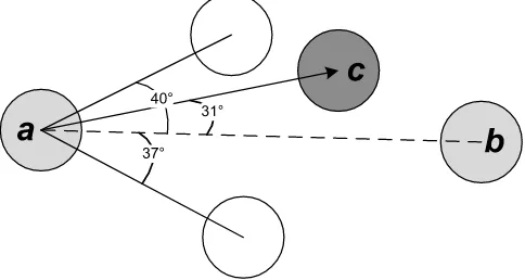
[image:1.595.317.559.456.585.2]When a source node a wants to send a packet to b which is out of its range, it has to choose an intermediate node c like the figure below
Figure 1 staying close to the straight-line joining the source and destination always reduces total path-length
Figure 2 sender must also make sure that it utilizes all its transmission range to the fullest capability so that hop count is reduced and delay is
minimized
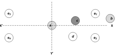
[image:2.595.38.281.64.165.2]If here c, d and e all are within the range of a then in the figure above forwarding to c is definitely not the best choice, rather e should be the more prolific one as it is closest to the destination. Consequently there are two properties of the intermediate node that in conjunction determines unequivocally which intermediate node should be chosen for forwarding- the node has to be closest to the straight-line between the source and destination, it should be furthest away from the source. According to this rule e will be chosen as the forwarding node. However there arises another issue, just as depicted in the figure below
Figure 3 depending on the angle and most distant node doesn’t always yield correct solution
According to the rule specified before nodes e1, e2, e3 and
e4 all are contender to be selected as the forwarding node
because they are all equidistant from the straight-line between a and b and they are also at the same distance from the source node a. But only e1 and e2 are legitimate choice, therefore there
has to be a mechanism to eliminate the choices e3 and e4. After
farther investigation it can be inferred that picking up not the node furthest from source rather closest to destination should solve the issue and eliminate e3 and e4 from the choice list.
Eventually the forwarding node selection strategy is – select the node that is closest to the straight-line between source and destination and closest to the destination. This forwarding node selection scheme is described as a mathematical model in the later sections.
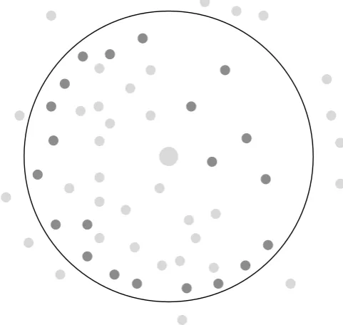
The main concern with MANET protocols is they tend to be processor intensive and there are quite a few reasons this is a big issue. First of all MANET has no fixed infrastructure to share the bulk of the workload. Therefore each node has to accomplish multidimensional responsibilities – disseminate node location coordinates, that is perform as the location server, maintain routes and respond to queries from other nodes, thirdly forward others packets to appropriate destinations and above all perform their own network related tasks. To make things more critical MANET devices are all wireless, constantly change their positions and all devices run on batteries and hence the chances are high that they will quickly drain their batteries. This will invalidate the forwarding scheme outlined before, at least for dense network. Typically in a dense network the area of the network surrounding a node looks as the following
Figure 4 random node distribution around a typical node. The deeply shaded ones are point of interest as the forwarding node
[image:2.595.37.279.330.407.2]Figure 5 circular zones to prioritize distant neighbors for forwarding
Now the forwarding node selection is not only dependent upon its distance from the source node but also on the angle between the straight-line joining the source and destination. Unfortunately this angle cannot be pre-computed because for different destination, the straight-line changes invariably and consequently the angle has to be recalculated. Obviously this is another hurdle the protocol must also overcome, because like distance calculation, intermediate angle calculation between two straight–line is also processor intensive. The protocol solves this issue by introducing similar approach as the circular zones. But to make this feasible the first task is to make the angle measurement system independent of the destination. This is accomplished by establishing a simple coordinate system around any node based on its original geographic coordinates, the longitude and latitude as depicted in the figure below
X X’
Y
Y’
Figure 6 dividing the angular area into quadrants
As we can see, previously all the angle calculations was based upon the straight-line joining the source and destination, but now there is a virtual coordinate system around the source node and the entire angular space of 360° is divided into four quadrants. This division of number four is significant and not unrelated to previous division of four circular zones. This must be stated here that this division of four circular zones or four quadrants is not predefined or rigid, rather the number can be altered or increased with respect to the density of the network. However for the present scenario four seems to be an optimal value. But there is a constraint on the number of division which is the number of circular zones and angular blocks must be equal. The rationale behind the constraint will be evident sooner than later, but currently stated just to maintain relevancy. Now coming to the point the X axis is parallel to
the geographic equator. As the node coordinates are known determining the equation for X axis straight-line is very much possible. The Y axis is perpendicular to the X-axis. Now when a node is registered as a neighbor and enlisted in one of the four circular zones, it’s another property is determined which is its quadrant it belongs to. Therefore now the list of the neighbors also maps the quadrant of the particular node with its priority value.
As most primary theories are discussed now, the working principle of the protocol can be clearly understood. When a node comes into existence the first thing it does is it finds its own coordinate with the help of the GPS [9]. More information about GPS [10], how it works and its feasibility [11] as a tool for MANET [12] is analyzed in details in several contemporaneous publications [13]. Then the node establishes the virtual quadrants and the circular zones. The node broadcasts a single hop HELLO packet. All the nodes within its radio range receives the HELLO packet and responds with their ID and coordinates. Using the neighbors coordinates and its own coordinate the node computes the distance of each neighbor. According to the distance the node groups its neighbors into circular zone. It also determines the quadrant each neighbor belongs to. The node then creates four lists of its neighboring nodes, each list already has a predefined priority, and the quadrant information is also stored along with the neighbors ID. Now at time of routing the source node first determines which quadrant the destination falls into. Then searches for a node in the outermost circular zone in the same quadrant. The first node it finds with matching quadrant, it forwards the packet to that node. Now finding a proper node in the appropriate quadrant is an optimum choice which is not likely to take place all the time. So therefore the protocol defines and utilizes a unique protocol as outlined in the following section.
II. RELIABLE AND DENSITY-AWARE ROUTING PROTOCOL FOR MOBILE AD HOC NETWORK WITH NOVEL POWER
CONSERVATION SCHEME
A. The Routing Protocol Algorithm:
To find the optimum forwarding node the routing protocol adheres to the following algorithm
a) The routing protocol defines a term range of deviation; it is the difference in optimum forwarding choice property and available forwarding choice property b) Initially the value of range of deviation is zero. In the
circular zone property, the optimum circular zone is the outermost circle. So the protocol only checks the outermost circle, not any other circle. If it finds some then it looks for the any node in the desired quadrant, the quadrant of the destination. The first matching node is selected for forwarding. If no node is found, no other quadrant is searched, as the range of deviation is now zero. So when the range of deviation is zero the protocol can only accept nodes in the outermost circular zone in the matching quadrant.
[image:3.595.44.275.488.598.2]zone that is in the desired quadrant, then for this node circular deviation is one, but angular deviation is zero. For both the nodes, summation of angular and circular deviation is same. In this case, the node with lesser angular deviation will be given priority and selected for forwarding.
d) The range of deviation is increased in the above manner until hopefully at least one optimum node is found. If no node is found the forwarding cannot proceed.
X
X’
Y
Y’
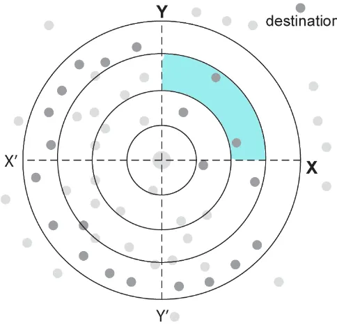
[image:4.595.314.556.53.283.2]destination
Figure 7 the circular zones and quadrant system together. The destination is labelled and the sender is at the center
Figure 8 the deeply shaded area is the best choice for forwarding. But no node belongs to that zone. Therefore range of deviation must be expanded.
[image:4.595.42.277.62.395.2]Here the range of deviation is zero
Figure 9 the range of deviation is expanded to one. So probable zone list has increased. The lightly shaded areas here are considered for forwarding. But because of the laws of the algorithm the zone in the same quadrant with
[image:4.595.315.557.333.566.2]the destination will be selected for forwarding
Figure 10 the colored area is the ultimate choice for forwarding here according to the algorithm. Any node in this zone can be selected for
forwarding
B. Mathematical Model Behind Forwarding
Let us consider the equator or any other straight-line as the base for all our calculations. Let the equation for that straight-line be
0
ax by
c
(1) Then the X axis should be parallel to this line. So X axis should have the same slope.Now the slope from the base straight-line equation is
a
m
b
[image:4.595.40.277.428.656.2](
a
)(x p)
y q
b
(2)This should be the equation for X axis. Now the equation for the Y axis should be the one passing through the node and perpendicular to the X axis. Let the simplified equation for X axis is
0
x
y
(3) Then its slope ism
The coordinate for the center node is as before (p, q). Then the equation for the Y axis will be
( )(x p)
y
q
(4)As the equation for and X and Y axis are now determined, the quadrant that any point belongs to can easily be calculated. When a node is registered as neighbor, its distance from the source is calculated. Let the coordinate or the source is (p, q) and the new node is (r, s) then their distance can be calculated using the following equation
2 2
(p r)
(q s)
d
(5)C. Adapting to the Effect of Density
As this has been stated repeatedly in the prior discussions, that MANET protocols must learn to adapt to unstable network circumstances. Generally the adaptation done in other protocols come from the entire network perspective. The problem with this approach is when the network parameters change all nodes must be updated with the new information. This process is very slow and itself pulls on heavy network overhead. Therefore the protocol in this paper takes a different approach. The adaptation is done on the local information of the nodes when new nodes are registered as neighbors. As it has been said before that the protocol mandates that no. of quadrants must equal the no. of circular zones. To adapt to density the node has a typical threshold for no. zones. Increase in no. of neighbor is related to the increase in density. With 0~5 nodes in the neighbors a node creates no circular or angular zone. The forwarding node selection becomes direct and accurate. When the no. of neighbor is 6~15, the node creates 2 circular zone and quadrants. With 16~30 nodes the node creates 3 zones, for 31~40 nodes 4 zones are created, for 41~50 nodes there are 5 zones, for 51~60 nodes there are 6 zones, for 61~80 nodes there are 8 zones. In this way the protocol adapts to different density with practically little or no network overhead induced.
D. Reliable Routing and Avoiding Bottlenecks
In ad hoc networks each node has to perform multi-faceted responsibilities. It is often the case that the network distribution is as such that a particular node is in a position that all other nodes uses it to forward packet or other routing information. In time this node becomes a bottleneck and the performance degrades. There might be another scenario that the node is on the edge of a hole in a network and therefore there are no forwarding nodes available, so if it receives a packet to forward, ultimately the packet will reach a dead-end. These are the long term information that grows over time. To take advantage of such routing hints the protocol also stores these information globally with the location information of each node. When a node involves in a forwarding step, if that
results in successful packet forwarding its trust factor increases and with each failure it decreases. Therefore when taking any forwarding decision each node also accounts for the intermediate nodes trust factor. The highest trust factor is one and the lowest is zero. If any node is in congestion it returns the packet to sender and invariably its trust factor decreases. Similarly in case of route failure or unavailability the trust property decreases. The inclusion of trust property significantly increases network reliability and reduces packet failure.
E. Minimization of System Power Rquirement
Recent researches focuses much on battery power. Because all optimization requires battery power, reducing power is a critical issue [14]. The protocol has quite a number of features to reduce battery drainage. The protocol calculates a neighbor’s distance only once that is during the period of hello packet exchange. Distance calculation involves square-root which is a very processor intensive task. The protocol also saves memory by not maintaining all the detailed information on all the neighbors like storing their exact position and double precision floating point distance could easily bloat up each nodes memory. But the protocol intuitively maintains list or hierarchy. This also save searching time, as there are more than one lists in general the protocol doesn’t have to go through all the lists all time. This saves searching time. Instead of calculating the actual angle the protocol maintains quadrants. This saves lots of processing power and comparison effort. The equation in between the straight-line and destination is not generated anymore, nor the distance between source and destination needs to be calculated, therefore processing resources is saved there as. The calculation of trust factor also reduces packet failure and retransmission efforts which is also a great addition to the protocol.
III. SIMULATION AND PERFORMANCE ANALYSIS
Figure 11 packet delivery ratio vs. no. of packets generated per sec. per node. Higher values are better. Packet delivery ratio drops with congestion
[image:6.595.315.562.59.256.2]or heavy workload
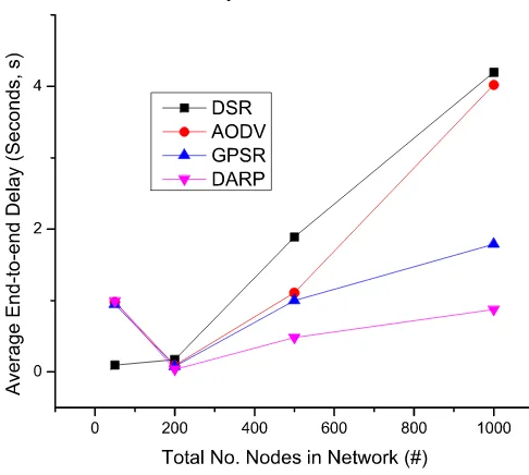
Figure 12 packet delivery ratio vs. total no. of nodes in the network. Packets per node and network area is kept constant. Again high network
density induces packet loss
[image:6.595.313.556.291.509.2]The simulation environment was set up for 50~1000 nodes with 1050 m by 1050 m of flat space, standard radio signal characteristics defined in NS-3 was utilized. For simulating mobility the random waypoint model of NS-3 was chosen. To test the adaptability of all the nodes the simulation was run in typically two configurations. First the total node number was constant but unique packets generated per second was gradually raised, it was very beneficial to observe how the protocols reacted to network congestion. The second scenario was set to check the protocols reaction to density change. Therefore packets generated per node and the overall network area remained constant while the total no. of nodes involved in the network was changed gradually. To analyze the relative performance of the protocol with comparative protocols is left to the consideration of the reader.
Figure 13 average delay, the average of the interval a packet spends to reach its ultimate destination. The lower the value the better is the
performance
Figure 14 comparative average end-to-end delay, like the figure before. Again it takes more time in a heavily congested area.
Figure 15 when a new data packet is created by a certain node, it is recreated several times by other nodes for forwarding. Besides there are
other control packets to run the protocol. Here the comparison is made between the total no. of any packet created in a network vs. the unique new
[image:6.595.36.273.297.497.2] [image:6.595.315.557.531.733.2]Figure 16 total packets vs. unique new packets, wrt. total no. of nodes in the network
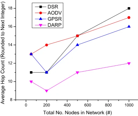
Figure 17 average hop count vs. packet generation rate. In common routine protocols with congestion hop count increases rapidly. But with location
based and greedy protocols it is not the same
Figure 18 another representation of average hop count vs. network congestion graph. Like figures before the node count changes while packets
per node and network area remain constant
IV. CONCLUSION
Due to the inherent nature of the MANET environment no routing protocol can be deemed as perfect. Therefore the main concern that dominated the design of the routing protocol was simplicity. Because of the dynamic nature of MANET to much calculation intensive optimization is sure fail. To avoid unnecessary calculation overhead always a simplified heuristic solution was introduced. Another major aspect of the protocol is the adaptability to changeable network parameters and making this change just with local information of the node. So there is little updating cost. There are several modification and enhancements are under active consideration, mostly to curb the effect of mobility. Those enhancements are kept for any future release of the protocol. For now on the scalable approaches outlined in this paper are expected to make a mark in the field of mobile ad hoc networks.
V. ACKNOWLEDGMENT
This work is part of a thesis research performed on ad hoc network topology. I am especially thankful to my adviser and institution as a whole for providing technical and informative support and advice on every steps to accomplish this task and make it successful.
VI. REFERENCES
[1] IEEE802.11ac: The Next Evolution of Wi-Fi Standards, May 2012, retrieved on September 16, 2012, http://www.qualcomm.com/media/documents/files/ieee802-11ac-the-next-evolution-of-wi-fi.pdf
[2] Science Reference Services, retrieved from http://www.loc.gov/rr/scitech/mysteries/global.html on March 28, 2014.
[3] S. Basagni, I. Chlamtac, V.R. Syrotiuk and B.A. Woodward, A distance routing effect algorithm for mobility (DREAM), in: ACM/IEEE International Conference on Mobile Computing and Networking (Mobicom '98) (1998) pp. 76–84.
[4] Jinyang Li, John Jannotti, Douglas S. J. De Couto, David R. Karger, and Robert Morris, A Scalable Location Service for Geographic Ad Hoc Routing, In Proceedings ACM Mobicom, Boston, MA (2000).
[5] X. Lin and I. Stojmenovi´c, Geographic distance routing in ad hoc wireless networks, Technical report TR-98-10, SITE, University of Ottawa (December 1998).
[6] Imrich Chlamtac, Marco Conti, Jennifer J.-N. Liu, Mobile ad hoc networking: imperatives and challenges, Ad Hoc Networks 1, Elsevier, pp. 13-64 (2003).
[7] E. Kranakis, H. Singh and J. Urrutia, Compass Routing on Geometric Networks, Proceedings of the 11th Canadian Conference on Computational Geometry pp. 51-54 (1999)
[8] J. Urrutia, "Routing with Guaranteed Delivery in Geometric and Wireless Networks," Handbook of
[image:7.595.35.277.530.734.2][10] GPS Accuracy, retrieved from http://www.gps.gov/systems/gps/performance/accuracy/ on March 28, 2014.
[11] Global Positioning System, Precise Positioning Service Performance Standard, February 2007, http://www.gps.gov/technical/ps/2007-PPS-performance-standard.pdf
[12] Global Positioning System, Standard Positioning Service Performance Standard, 4th Edition, September 2008, http://www.gps.gov/technical/ps/2008-SPS-performance-standard.pdf
[13] Young-Joo Suh, Won-Ik Kim, Dong-Hee Kwon, GPS-Based Reliable Routing Algorithms for Ad Hoc Networks, The Handbook Of Ad Hoc Wireless Networks, CRC Press, pp. 350-363 (2003)
[14] Wireless Networks and Mobile Computing, pp. 393 – 406, John Wiley and Sons, 2002.
[15] D.B. Johnson, D.A. Maltz, Y.-C. Hu, J.G. Jetcheva, The dynamic source routing protocol for mobile ad hoc networks (DSR), Internet draft, draft-ietf-manet-dsr-07.txt (2002) [16] C.E. Perkins, E.M. Royer, S.R. Das, Ad hoc on-demand
distance vector (AODV) routing, Internet draft (2001)
[17] GPSR: greedy perimeter stateless routing for wireless networks, Brad Karp, H. T. Kung, Proceeding MobiCom '00 Proceedings of the 6th annual international conference on Mobile computing and networking, Pages 243-254, ACM New York, NY, USA 2000