Zero One Sampling System

1556

Zero One Sampling System

Arumainayagam S.D1, Vennila J2

DepartmentofStatistics1 Government Arts College,

Coimbatore – 641 018, Tamil Nadu, India. Email: [email protected]

DepartmentofStatistics2 KMCH College of Pharmacy,

Coimbatore – 641 048, Tamil Nadu, India Email: [email protected]

Abstract- This paper introduces a new switching system meant for costly and destructive testing. Measures of

performance, designing of system for various entry parameters and comparison with existing plans are given.

Index Terms-Acceptance Sampling System, Quick Switching System, Destructive Testing.

1. INTRODUCTION

Dodge (1967) introduced a new sampling system called “Quick Switching System” (QSS-1) for attributes acceptance sampling plan, involving both normal and tightened plans. The application of the system is as follows:

1. Adopt a pair of sampling plans, a normal plan (N) and tightened plan (T), the plan T to be tightened OC curve wise than plan N.

2. Use plan N for the first lot (optional): can start with plan T; the OC curve properties are the same; but first lot protection is greater if plan T is used. 3. For each lot inspected; if the lot is accepted, use

plan N for the next lot and if the lot is rejected, use plan T for the next lot‟.

Further, Romboski (1969) has developed two QSSs, namely QSS (n, cN, cT) and QSS(n, kn, c0).

Soundararajan and Arumainayagam (1988) provided the tables for the selection of modified QSS. Soundararajan and Arumainayagam (1990, 1991, 1992, 1994 and 1995) have developed QSS using single, double and repetitive sampling plans as reference plans. Soundararajan and Arumainayagam (1992) developed systems based on QSS for products involving costly and destructive testing. Suresh (1993) has proposed a procedure for selection of QSS indexed through various quality limits.

Arumainayagam and Uma (2008)

constructed the tables for matched single, double and multiple sampling plans using QSS. Suresh and Kaviyarsu(2008) studied quick switching system with conditional group sampling plan as reference plan.

Arumainayagam and Uma (2009 and 2013) have developed QSS using single sampling plan as

reference plan with weighted Poison distribution. Suresh and Jayalakshmi (2009) have developed QSS with special type of double sampling plan as reference plan.

Arumainayagam and Uma (2011) have studied QSS using triple sampling plan as reference plan. Uma and Nandhinidevi (2015) have studied the quick switching system with fuzzy logic system in Poisson distribution. Uma and Gunasekaran (2016)

have developed QSS Zero Inflated Poisson

Distribution as reference plan and compared ZIP with Poisson distribution for the purpose of consumer protection. Uma and Ramya (2017) studied QSS with double sampling plan fuzzy binomial distribution as the baseline distribution. Divya and Arumainayagam (2018) studied QSS using multiple sampling plans as reference plan.

1557 2. ZERO ONE SAMPLING SYSTEM

This system is designated as zero one sampling system ZOSS (n; k), where the normal double sampling has the parameters of n1=n2=n, c1=0

and c2=1 and tightened single sampling has the

parameters kn, k ≥ 1.

2.1. Conditions for Application

i. The product to be inspected is of a series of successive lots produced by a continuing process. ii. Normally, lots are expected to be essentially of the same quality.

iii. Lots are submitted substantially in the order of production.

iv. Inspection is by attributes, with quality defined as the fraction non-conforming.

2.2. Operating Procedure

Step 1: From a lot, take a random sample of size n and count the number of defectives x1.

(i) If x1 = 0, then accept the lot, repeat step 1

for the next lot.

(ii) If x1 > 1, then reject the lot and continue

step 2 for the next lot.

(iii) If x1 = 1, then take a second random

sample of size n form the same lot, and count the number of defectives x2.

(iv) x1 + x2 = 1, then accept the lot and repeat

step 1 for the next lot

(v) x1 + x2 > 1, then reject the lot and go to

step 2 for the next lot.

Step 2: From the next lot, take a random sample of size kn at tightened inspection level and count the number of defectives x.

(i) If x ≤ 0, accept the lot and go to step 1 for the next lot.

(ii) If x > 0, reject the lot and repeat step 2 for the next lot.

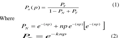
3. MEASURES OF PERFORMANCE The OC function of ZOSS (n; k) is given below

T N

T a

P

P

P

p

P







1

)

(

Where

PN = Proportion of lots expected to be accepted when

using normal double sampling plan

PT = Proportion of lots expected to be accepted when

using tightened single sampling plan

Under the assumption of Poisson Model (Hamaker and Van Strik (1995)), values of PN and PT are given

by

) 2 ( )

(np np

N e npe

P    

knp

T

e

P



3.1. Properties of the OC Curve

1. Figures. 1 and 2 give the normal, tightened and composite OC curve of ZOSS. The composite OC curve lies between normal and tightened OC curves. For good quality, the normal plan has more probability being applied in the system and hence it is closer to the composite OC curve. From these curves; it is observed that, when comparing the composite OC curve with its corresponding normal and tightened OC curves, it is in better shape than the other curves. 2. Figures 3 and 4 give a set of composite OC curves. In these curves, the normal plan is fixed and in the tightened plan k is allowed to increase. That is tightening is made severe. It is observed that as the value of p increases, the OC curve approaches to the shape of an ideal OC curve.

Figure 1: Normal, Tightened and Composite OC curves of ZOSS

Figure 2: Normal, Tightened and Composite OC curves of ZOSS

1558 Figure 4: Composite OC curves of ZOSS

4. ASN

Based on the work of Stephens and Larson (1967), the ASN function for the ZOSS is given below

ASN = ASNN PN + ASNT PT (3)

Where

ASNN = ASN of Normal double sampling plan

ASNT = ASN of Tightened single sampling plan

PN = the expected proportions of lots inspected during normal inspection

PT = the expected proportions of lots inspected during tightened inspection

The ASNs of the normal double and tightened single sampling plans of ZOSS (n, k) are given by

On substituting equations (4) and (5) into equation (3), we get the ASN of ZOSS (n, k) as

Where ATIN and ATIT are the average total inspection

of the normal double sampling plan and tightened single sampling plan respectively. From Duncan (1986), ATIN and ATIT for ZOSS (n; k) under Poisson

Where N is the lot size and substituting equations (5), (8) and (9) into equations (7), we get the ATI of ZOSS

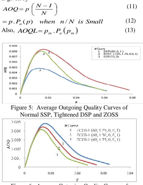
Assuming the nonconforming units are replaced by good units in samples taken from accepted lots and also that nonconforming units are completely replaced in rejected lots, the average outgoing quality of ZOSS is given by

Figure 5: Average Outgoing Quality Curves of Normal SSP, Tightened DSP and ZOSS

Figure 6: Average Outgoing Quality Curves of Normal SSP, Tightened DSP and ZOSS

From the above AOQ curve,

1559

steps are to be followed:

1. Compute p2/p1 = 0.09 / 0.01 = 9.00

6.3. Designing system given AQL and AOQL

Table 5 can be used to design ZOSS (n; k) for specified values of AQL and AOQL.

Example

6.4. Indifference Quality Level and h0

Table 5 can be used to design ZOSS (n; k) indexed by point of control and point of control.

Example

parameters, value of np0 is 0.6860. The sample size of

normal double sampling plan is obtained as n = np0 / n

= 0.6860 / 0.02 ≈ 34. The designed system is ZOSS (34; 1.65, 0; 0, 1).

6.5. Calculating AOQL of the system

Table 5 provides the npm and nAOQL values for

ZOSS (n; k). This table can be used to determine npm

and nAOQL of a system.

Example:

Determine the pm and AOQL of ZOSS (34; 1.65; 0; 0, 1). From Table 5, corresponding to k=1.65, nAOQL = 0.0109 and npm = 3.4991. so AOQL = nAOQL / n =

0.0109 / 34 = 0.0003% and pm = npm / n = 3.4991 / 34

= 0.10%.

6.6. Conversion of Parameters

For ZOSS (n; k), if p1=0.02, p2=0.04, α=0.05 and

β=0.10, the system satisfying the requirements can be obtained from Table 5 as n = 34, k= 1.65, c = 0, c1 = 0

So,AOQL = nAOQL/n = 0.0109/34 = 0.0003 p0 = np0 / n = 0.1799/34 = 0.0053.

So, when p1=0.02, α = 0.05, p2 = 0.04 and β = 0.10,

the other similar sets of parameters are given by 1. p1 = 0.02 (α = 0.05) and AOQL = 0.0003

2. p0 = 0.0053 and h0 = 1.2020.

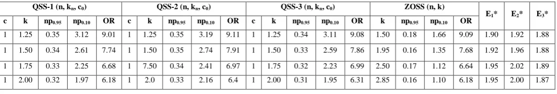
7. COMPARISON & CONCLUSION

Four QSS-1 (n, kn, c0), QSS-2 (n, kn, c0), QSS-3 (n, kn,

c0) and their equivalent ZOSS (n, k) values are given

1560 basis for „matching‟. QSS-1 (n, kn, c0), QSS-2 (n, kn,

c0), QSS-3 (n, kn, c0) plan values are taken from

Soundararajan and Arumainayagm (1988). From this table, it is observed that the new system requires lesser sample size and it‟s shown to be more efficient than the existing one.

8. CONSTRUCTION OF TABLES

The OC function of ZOSS (n; k) is given below

ratio p2/p1 is calculated and that values are tabulated in

Table 4 for assumed values of α and β. Assuming nAOQ=np*Pa(p), for given values of c, c1, c2, the

values of npm which maximise nAOQ can be obtained

from equation (1). Values of npm and nAOQL are

[1] Arumainayagam SD (1991): “Contributions to the study of Quick Switching System (QSS) and its Applications”. Doctoral dissertation, Bharathiar University, Coimbatore, Tamil Nadu, India. [2] Arumainayagam SD and Divya (2018): “Designing

and Selection of Quick Switching Multiple

Sampling System – Acceptance Number

Tightening”, International Journal of Pure and Applied Mathematics, Vol. 119, No. 17, pp. 589-602.

[3] Arumainayagam SD and Uma G (2008): Construction of Matched Quick Switching Single

Double and Multiple Sampling Systems,

International Journal of Statistics and

Systems;2008, Vol. 3 Issue 2, p147.

[4] Arumainayagam SD and Uma G (2009): Construction and selection of quick switching multiple sampling system-sample size tightening, Indian Association Productivity and Quality Journal, 2009, vol.34, No.2.

[5] Arumainayagam SD and Uma G (2011): Construction and Selection of Quick Switching Multiple Sampling System – Sample Size Tightening, Quality Control and applied statistics, Vol.56, No.1-2, pp.65-66.

[6] Arumainayagam SD and Uma G (2013): Construction and selection of quick switching system using weighted Poisson distribution-sample size tightening, Indian Association Productivity and Quality Journal, 2009, vol.34, No.2.

[7] Arumainayagam SD and Uma G (2009): Construction and Selection of Quick Switching System Using Weighted Poisson Distribution,

International Journal of Statistics and

Systems;2009, Vol. 4 Issue 2, p127.

[8] Dodge, H. F. (1965): “Evaluation of a Sampling Inspection System having Rules for Switching Between Normal and Tightened Inspection”, Technical Report No.14, The Statistics Center, Rutgers – The State University, New Brunswick, New Jersey.

[9] Duncan, A. J. (1986): Quality Control and Industrial Statistics, 5th Edition, Homewood, Illinois, Richard D. Irwin.

[10] Hamaker, H.C. and Van Strik, R. (1955): The Efficiency of Double Sampling for Attributes, Journal of the American Statistical Association, Vol.50, pp. 830-849.

[11] Jayalakshmi, S. (2009): “Contribution to the Selection of Quick Switching System and related sampling plans”, Ph.D Thesis, Department of Statistics, Bharathiar University, Coimbatore, Tamil Nadu, India.

[12] Romboski, L. D. (1969): An Investigation of Quick Switching Acceptance Sampling Systems, Ph.D Thesis, Rutgers- The State University, New Brunswick, New Jersey.

[13] Soundararajan V and Arumainayagam SD (1989): “An Extension of Some Switching Procedures Used in Sampling Inspection”, International Journal of Quality and Reliability Management, Vol.06 (5) pp.141-153.

[14] Soundararajan V and Arumainayagam SD (1990): “Construction and Selection of Modified Quick Switching System”, Journal of Applied Statistics. Vol.17 (1), pp. 83-114.

[15] Soundararajan V and Arumainayagam SD (1990a): A Generalized procedure for Selection of Attribute Double Sampling plan, Communication in Statistics-Simulation and Computation, Vol.19, No.3, pp.1015-1034.

[16] Soundararajan V and Arumainayagam SD (1990b): Construction and Selection of Modified Quick Switching System, Journal of Applied Statistics, Vol.17, No.1, pp.83-114.

[17] Soundararajan V and Arumainayagam SD (1992):

Conditional double sampling

system Communications in Statistics - Theory and Methods. 21: 2019-2044.

1561 Destructive Testing, Sankaya, Series B–Part I,

Vol.54, pp.1-12.

[19] Soundararajan V and Arumainayagam SD (1992): Some sampling plans with identical operating characteristic curves Journal of Applied Statistics. 19: 141-153.

[20] Soundararajan V and Arumainayagam SD (1994): Construction and selection of quick switching double sampling system-acceptance number tightening Communication in Statistics – Theory and Methods 23, 7 2079-2100.

[21] Soundararajan V and Arumainayagam SD (1995): Construction and evaluation of matched quick switching systems International Journal of Applied Statistics vol.22, no.2, pp. 245-251. [22] Soundararajan V and Arumainayagam SD

(1995): Construction and Selection of quick switching system sample size tightening, Journal of applied Statistics, Vol.22, No.2, 1995, pp. 105-119.

[23] Soundararajan V and Arumainayagam SD (1995): Quick switching double sampling system indexed by the crossover point Communications in Statistics - Simulation and Computation. 24: 765-773.

[24] Stephens, K. S. and Larson, K. E. (1967): An evaluation of the MILSTD- 105D Systems of Sampling Plans, Industrial Quality Control, Vol.23, N0.7, pp.310-319.

[25] Suresh, K. K. (1993): A Study on Acceptance Sampling using Acceptable and Limiting Quality Levels, Ph.D., thesis, Department of Statistics, Bharathiar University Coimbatore, Tamilnadu, India.

[26] Suresh, K. K. and Kaviyarasu, V. (2013): Contribution of the Study on Quick Switching System Through Incoming and Outgoing Quality Levels, Ph.D Thesis, Department of Statistics, Bharathiar University, Coimbatore, Tamil Nadu, India.

[27] Uma G and Gunasekaran K (2016): “The Construction and Selection of Quick Switching

System Using Zero – Inflated Poisson

distribution”, International Journal of Advanced Engineering and Global Technology I Vol-04, Issue-02, pp.

[28] Uma G and Ramya K (2017): “Determination of Quick Switching Double Sampling System by Attributes under Fuzzy Binomial Distribution – Sample Size Tightening”, ICTACT Journal on Soft Computing, Vol 08, ISS. 01, pp.1539-1543 [29] Vennila J and Arumainayagam SD (2017),

“Construction and Selection of Quick Switching Single Double Sampling System”, International Journal of Applied Mathematics and Statistics, Vol. 56 (6), pp. 124 – 137.

1562

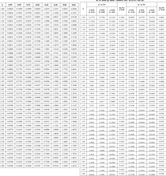
Table 3: Values of np tabulated against k for the given

1563 Table 5: Parametric values for ZOSS (n, k)

k h0 npm nAOQL

AOQL/p1

for 0.05 np1

1.00 0.99 5.7581 0.0102 0.0535 0.1909

1.10 1.03 5.2356 0.0165 0.0873 0.1891

1.15 1.05 5.0086 0.0158 0.0839 0.1882

1.20 1.07 4.8006 0.0151 0.0807 0.1873

1.25 1.08 4.6094 0.0145 0.0778 0.1865

1.30 1.10 4.4329 0.0139 0.0751 0.1856

1.35 1.11 4.2696 0.0134 0.0725 0.1848

1.40 1.13 4.1180 0.0129 0.0702 0.1839

1.45 1.15 3.9770 0.0124 0.0680 0.1831

1.50 1.16 3.8454 0.0120 0.0659 0.1823

1.55 1.17 3.7225 0.0116 0.0640 0.1815

1.60 1.19 3.6072 0.0112 0.0622 0.1807

1.65 1.20 3.4991 0.0109 0.0605 0.1799

1.70 1.22 3.3973 0.0105 0.0588 0.1791

1.75 1.23 3.3015 0.0102 0.0573 0.1784

1.80 1.24 3.2110 0.0099 0.0558 0.1776

1.85 1.25 3.1254 0.0096 0.0545 0.1769

1.90 1.27 3.0445 0.0094 0.0531 0.1761

1.95 1.28 2.9677 0.0091 0.0519 0.1754

2.00 1.29 2.8948 0.0089 0.0507 0.1747

2.05 1.30 2.8255 0.0086 0.0495 0.1740

2.10 1.31 2.7596 0.0084 0.0484 0.1733

2.15 1.32 2.6967 0.0082 0.0474 0.1726

k h0 npm nAOQL

AOQL/p1

for 0.05 np1

2.20 1.33 2.6368 0.0080 0.0464 0.1719

2.25 1.34 2.5795 0.0078 0.0454 0.1712

2.30 1.35 2.5248 0.0076 0.0445 0.1706

2.35 1.37 2.4724 0.0074 0.0436 0.1699

2.40 1.38 2.4223 0.0072 0.0427 0.1693

2.45 1.39 2.3742 0.0071 0.0419 0.1686

2.50 1.39 2.3281 0.0069 0.0411 0.1680

2.55 1.40 2.2838 0.0068 0.0403 0.1674

2.60 1.41 2.2412 0.0066 0.0396 0.1667

2.65 1.42 2.2002 0.0065 0.0389 0.1661

2.70 1.43 2.1608 0.0063 0.0382 0.1655

2.75 1.44 2.1228 0.0062 0.0375 0.1649

2.80 1.45 2.0862 0.0061 0.0369 0.1643

2.85 1.46 2.0509 0.0059 0.0363 0.1637

2.90 1.47 2.0169 0.0058 0.0356 0.1631

2.95 1.48 1.9840 0.0057 0.0351 0.1625

3.00 1.48 1.9522 0.0056 0.0345 0.1620

Table 2 – Comparison of Single Sampling, Double Sampling and ZOSS

QSS-1 (n, kn, c0) QSS-2 (n, kn, c0) QSS-3 (n, kn, c0) ZOSS (n, k)

E1* E2* E3*

c k np0.95 np0.10 OR c k np0.95 np0.10 OR c k np0.95 np0.10 OR k np0.95 np0.10 OR

1 1.25 0.35 3.12 9.01 1 1.25 0.35 3.19 9.11 1 1.25 0.34 3.11 9.08 1.50 0.18 1.66 9.09 1.90 1.92 1.88

1 1.50 0.34 2.61 7.74 1 1.50 0.35 2.74 7.91 1 1.50 0.33 2.59 7.86 1.95 0.16 1.35 7.68 1.92 1.96 1.88

1 1.75 0.33 2.25 6.68 1 7.50 0.34 2.41 6.97 1 1.75 0.32 2.23 6.99 2.50 0.17 1.12 6.64 1.95 2.02 1.89 1 2.00 0.32 1.97 6.18 1 2.0 0.33 2.16 6.4 1 2.00 0.31 1.95 6.31 2.85 0.16 1.10 6.18 1.95 2.00 1.87

Where

*E1 = np0.95 of QSS-1(n, kn, c0) / 0.95 of ZOSS (n, k)

*E3 = np0.95 of QSS-3(n, kn, c0) / np0.95 of ZOSS (n, k)