in Two-Stage Cluster Sampling
Nelson Kiprono Bii
Strathmore University, Nairobi, Kenya [email protected]
Ouma Christopher Onyango
Strathmore University, Kenyatta University, Kenya [email protected]
Abstract
Estimation of finite population parameters has been an area of concern to statisticians for decades. This paper presents an estimation of the population mean under a model-assisted approach. Dorfman (1992), Breidt and Opsomer (2000) and Ouma et al (2010) carried out the estimation of finite population total on the assumption that the sample size is large and the sampling distribution is approximately normal. Unlike their researches, this paper considered a case when the sample size is small under a model-assisted approach. A model-assisted regression model was considered in a case where the cluster sizes are known only for the sampled clusters in order to predict the unobserved part of the population mean. Under mild assumptions, the proposed estimator is asymptotically unbiased and its conditional error variance tends to zero. Simulation studies show that model assisted estimation performs better than model based estimation of a finite population mean in a case where the sample size is small.
Keywords: Model-assisted surveys, Non-parametric inference, Two-stage cluster sampling.
1.1 Introduction
Sample surveys are concerned with obtaining desired information from a population. In sample survey methods, some portion of the population called a sample is used to make inferences about the entire population.
Every nation in the world uses surveys to estimate their rates of unemployment, basic prevalence of immunization against diseases, opinions about the central government, intentions to vote in an upcoming election, and people’s satisfaction with goods and services that they purchase among other application areas. Surveys aid in tracking global economic trends, the rate of inflation in prices, and investments in new economic enterprises (Shewhart, 2004).
1.2 Background of the Problem
Model based methods in estimation of population parameters assume that there is an underlying model that generate survey units. However, if the assumed model is incorrect, the estimators of population parameters will certainly be incorrect. To address this problem, we wish to implement non-parametric approach to estimation of population mean then obtain a model that will be used to generate survey values given in finite populations in two stage cluster sampling. Model- assisted estimation of population total has been considered by Breidt and Opsomer (2000) under the assumption that the sample size is large and the sampling distribution is approximately normal. However, this is not always the case. In this study we consider a situation when the sample size is small and develop an estimator for estimating population mean.
In particular, the problem is to estimate the population mean defined as
̅ ∑
1.3 Summary of the paper
The rest of the paper is organized as follows: section 2 gives a summary of the two stage cluster sampling that we proposed to use. In section 3 we introduce the estimator for the finite population mean in two stage cluster sampling. In section 4 we look at the asymptotic properties of the proposed estimator. In section 5 we give the conclusion of our paper.
2. Review of Two Stage Cluster Sampling
Consider a finite population of primary sample units (PSU’s) or clusters labelled i.e where is a known number. Let , be the number of secondary sampling units(SSU’s) in the PSU.
Let be the value of the survey variable for the SSU belonging to the PSU. We further assumed that the auxilliary data are known for all the selected clusters and the population elements. The non-sampled units are not known and we therefore use the auxiliary information together with the sampled units of the survey variable to estimate the non-sampled part of the population. We proposed to estimate the population mean defined by equation (1.1). In this paper, we generate the survey values in the cluster by the modelgiven by
3. Proposed Estimator of the Population Mean
The population mean to be estimated is given by equation (1.1). The non-sampled survey values of the population are unknown. We therefore use the sampled units of the population together with the model defined in equation (2.1) to estimate the non-sampled part of the population mean. The proposed estimator is given by
̅̂ { ∑ ̂
}
4. Properties of the Proposed Estimator
4.1 Asymptotic Unbiasedness of the Estimator
The estimator of population mean is given by
̅̂ { ∑ ̂
}
{ ∑
}
Denoting the initial sampling weights by which is equal to the inverse of their selection probabilities i.e. probability of including unit from cluster in the sample, we have:
̅̂ { ∑ ∑
}
{ ∑ ∑ ̂
}
But as shown by Ouma et al (2010), , therefore the proposed estimator for the population mean becomes
( ̅̂) [ ∑ ∑ ̂
]
[∑
] ∑ * ̂ +
[∑
] ∑ [ ̂ ]
But
Since
Then
( ̅̂) [∑
]
Let the sampling weights of the primary sampling units be given by
( )
Rupert (2003) applied as a basis and suggested that the sampling weights in this kind of survey can be computed using
( )
( ) ⁄
Where is the number of times the primary sampling unit is chosen. Thus using this procedure, it follows that
( ̅̂) (
)
⁄
[∑
]
But since we sample with replacement we have ; Rao and Wu (1998) observed that there is considerable benefit and little loss in choosing ; therefore we put , so that
( ̅̂) (
)
⁄
[∑
]
[ ] ⁄ [∑
]
Let the initial sampling weights defined in ) be given by the kernel weights:
( )
( )
∑ ( )
Where
∑
Using ) we have
( ̅̂) [ ] ⁄ ∑ ( ).
( )
∑ ( )
/
Let
( ̂ ) ( )
be the kernel estimator of ( ) then
( ̅̂) [ ] ⁄
∑
0 ( )
( )
( ̂ )
1
This consequently gives us
( ̅̂) ( )
⁄
∑ [ ( ( ))]
( )
[ ( ̂ )]
We make the following substitutions:
}
( ̅̂) (
)
⁄
∑ [ ( ) ]
[ ( ̂ )]
Using substitutions in (4.19), from equation (4.20) we have
[ ( ̂ ) ] 0 ∑ ( )
1
( ) ∫ ∑ ( ) ( ) ( )
( ) ∫ ∑
Where [ ( ̂ ) ] is the conditional mean of ( ̂ ) given the auxiliary values of
.
We let ( ⁄ ) where is a kernel and is a chosen bandwidth. In addition is a symmetric density function such that
Since the relationship between the conditional mean and the selected bandwidth is too complex to establish we utilize the following theorem whose proof is given in Dorfman (1992).
Theorem: Let be a symmetric density function with ∫ and ∫ , assume that and increase together such that with
, assume sampled and non-sampled values of are in the interval [ ] and are generated by densities and respectively both bounded away from zero on [ ] and assumed to have continuous second derivatives. Iffor anyvariable Z, and , being a random variable and an observation, then
( ), where is an order of a term with elements.
From expression let ( ̂ ) i.e
( )
Then
[ ( ̂ )⁄ ] ∑ * ( )+
( ) ∑ ∫ ( )
Using the substitution
( )
And applying Taylor’s series expansion about a point we get
[ ( ̂ )⁄ ] ( ) ( )
[ ( ̂ )⁄ ] ∑ * ( )+
∑ [ * ( )+ * ( )+ ]
( ) ∑ [ * ( )+ * ( )+ ]
( ) ∑ ,∫ ( ) [∫ ( ) ]
Applying Taylor’s series expansion about a point on , we have
[ ( ̂ )⁄ ]
∑ * (
) ∫ ( ) ∫
(
) ∫ ( ) ∫
+
By the theorem stated above, this reduces to
[ ( ̂ )⁄ ]
[ ( ̂ )⁄ ] [ ( ̂ )⁄ ] 0 [ ( ̂ )⁄ ]1
The second term in equation (4.37) is given in equation (4.36), we therefore need to
evaluate [ ( ̂ )⁄ ] as follows:
[ ̂ ( )⁄ ] [ .∑ ( )
/ ]
[( ) ∑ ( ) ∑ ( )
]
But
[∑ (
)
⁄
] ∑ ∫ [ (
)
⁄ ]
( )
Applying the substitutions in (4.19) equation becomes
[∑ (
)
⁄
] ∑ ∫
Using Taylor’s series expansion about point in equation we get
[∑ (
)
⁄
]
∑ ∫
, ( ) ( )
( )
-
and
∑ ∑ ( ) ( )
∑ ∑ ∫
∫
Expanding the right hand side of equation we get
∑ ∑ * ( ) ∫ ( ) ∫ ( ) ∫
+
Therefore
∑ ∑ ( ) ( )
∑ ∑ * ( ) ( ) + * ( )
(
) +
by the above theorem.
This leads to
[ ( ) (
) ( ) ]
* ( ) ( ) +
Equation (4.46) leads to
∑ ∑ ( ) ( )
* ( )
+
Using this result in equation gives
[∑ (
)
⁄
]
* (
) ∫ ( ) ∫
∫
+
This simplifies to
[∑ (
)
⁄
]
* (
) ∫ ( ) ∫
∫ +
Therefore
[ ( )]
∫
∫ ∫
[ ] [
]
Thus we get
[ ( )] * + [(
) ] [ ]
Hence
[ ( ̂ )⁄ ] [ ]
From equation (4.20)
( ̅̂) ̅ ( ) *
As b , and for n small,
( ̅̂) ̅
And therefore the proposed estimator is asymptotically unbiased.
4.2 The Bias of the Proposed Estimator
The bias of the proposed estimator is given by
( ̅̂) ̅
( ̅̂) ̅ [ { ∑ ∑
} ∑
]
∑ ( ) ∑
∑
But
Hence
∑
( ̅̂) ̅ ∑ ( )
∑
But the inclusion probability in two-stage cluster sampling is given by
Therefore
( ̅̂) ̅ ∑ ( )
∑
We have
∑
Since
∑
( ̅̂) ̅ ∑ ( )
∑
As n becomes small the bias asymptotically tends to zero i.e
( ̅̂) ̅
4.3 Asymptotic Error Variance of the Proposed Estimator
[ ( ̅̂) ̅⁄ ]
( ̅̂) ̅
( ̅̂) ( )
due to i.i.d of auxiliary variables.
But
( ̅̂) [ (
)
⁄
∑ [ ( ( ))]
( )
[ ( ̂ )] ]
(
) ∑ * [ ( ̂ )]
+
( ( ))
(
) ∑ * [ ( ̂ )]
+
( )
Substituting equation (4.71) in equation (4.68) we get
[ ( ̅̂) ̅⁄ ]
( )
(
) ∑ * [ ( ̂ )]
+
( )
But as shown above, the conditional variance of ( ̂ ) is given by i.e
[ ( ̂ )⁄ ] [ ]
Which tends to zero as b , and hence the second term on the right of equation (4.72) vanishes. Therefore the error variance becomes
Table 1: Summary of the Mean Squared Error Values (MSE)
The table below shows the results of the mean squared errors (MSE) of the estimators of the finite population mean in two stage cluster sampling at different bandwidths.
Bandwidth Model-Assisted Model-Based
0.001 0.006646769 4.328651
0.002 0.001167328 4.071455
0.003 0.09797738 5.799239
0.004 0.2305878 4.33418
0.005 0.1958319 6.575275
0.006 0.1321953 5.486596
0.007 1.758383 4.897115
From Table 1 above we observe that at different bandwidths considered, the mean squared errors obtained in estimating population mean using the model-assisted estimator are significantly smaller than those incurred in using model-based estimator when the sample size is small i.e when n < 30 as used in the empirical study.
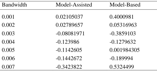
Table 2: Summary of the bias for the Two Estimators
Bandwidth Model-Assisted Model-Based
0.001 0.02105037 0.4000981
0.002 0.02789657 0.05316963
0.003 -0.08081971 -0.3859103
0.004 -0.123986 -0.1279632
0.005 -0.1142605 0.001984305
0.006 -0.1442672 -0.189994
0.007 -0.3423822 0.5324499
From Table 2 above we observe that the bias associated with the model assisted estimator increases insignificantly while that of model based estimator fluctuates. However, the bias due to model assisted estimator is comparatively low with respect to that of model based estimation at the different bandwidths considered.
It can be noted also that there is a trade-off between these two approaches as illustrated by the graphs. So none of the approaches is overally better but they can be compared at specific bandwiths.
5. Conclusion
population mean with the proposed estimator. Empirical results show that model-assisted approach performed better than model-based approach when the sample size is small. Comparison was done on the basis of the mean squared errors and biases of the two estimators.
References
1. Dorfman, A.H (1992). “Non-Parametric Regression for Estimating Totals in Finite Populations”. Proceedings of the Section on Survey Research Methods, American Statistical Association 622-625.
2. Breidt, F.J., and Opsomer, J. D. (2000). Local Polynomial Regression Estimators in Survey Sampling. The Annals of Statistics, 28, 1026-1063.
3. Ouma et al (2010). Generalized Model Based Confidence Intervals in Two Stage Cluster Sampling. Far East Journal of Statistics, 171-184.
4. Shewhart, A.W (2004). Properties and Use of Shewhart Method. Sequential Analysis, 2007, 26, 171-193.
5. Ruppert, et al (2003), Transformations and Weighting In Regression, London: Chapman and Hall.