AN EFFECTIVE JAMMERS CANCELLATION BY MEANS OF A RECTANGULAR ARRAY ANTENNA AND A SEQUENTIAL BLOCK LMS ALGORITHM: CASE OF MOBILE SOURCES
B. Atrouz
EMP, B. P. 17
Bordj El Bahri, Algiers, Algeria
A. Alimohad
University of Medea Medea, Algeria
B. A¨ıssa
INRS-´EMT
University of Quebec Quebec, Canada
Abstract—Adaptive array processing algorithms have received much attention in the past four decades. Modern radars have to consider various sources of noises and interferences for accurate and real time detection. In addition to interferences arising between the target and receiver, such as clutter and jammers, the use of the conventional techniques applied to the jammers cancelation in radars systems, especially when sources to cancel are moving (i.e., a dynamic environment as it is usually the case for air-and space-based radar), requires an adaptive arrays of several hundreds and/or thousands of elements. These methods are inefficient because of the large amount of data that describes the problem, which can limit considerably the achievement of the optimal performances due to the great computational complexity, costs and the very long time of both convergence and tracking. In this paper, we propose the study of a newly optimized algorithm, based on the known Least Mean Square (LMS) method due to its simplicity and effectiveness especially when work is driven toward the moving target tracking. Our proposed
algorithm contains two main issues, (i) the use of partial adaptively scheme and (ii) the use of the block processing method. We present here our performances in the improvement of the signal to interference plus noise ratio (SINR) obtained due to these two aspects in cancelation of jammers and tracking. Since all the signal transformations are simple and straightforward, good matching between these results was achieved, and our new process can be significantly faster than the LMS algorithm while its effectiveness is well comparable to that when the LMS algorithm is used directly.
1. INTRODUCTION
The use of the adaptive array processing techniques to circumvent and/or to cancel the intentional or unintentional interference signals is largely employed. The main advantage of using an adaptive array is its ability to track variations in the noise environment due to factors such as the movement of the array or jammers. In addition, depending on the algorithm employed, an adaptive array may also be able to compensate for the use of nonideal physical components such as radio antennas. Habitually, the effect of using these nonideal components is equivalent to that of having some unknown perturbations on the noise environment. An adaptive beamformer is collection of sensor elements whose outputs are combined by iteratively adjusted weight vector so as to pass a desired signal with minimum distortion while rejecting interfering signal. Since this form of array processing provides system antijam performance, it has become an essential requirement for the military and high resolution radars, communications and navigation systems [1–11].
LMS Implementation Outlines
steering beamformers [14] can be employed as the underlying array processing structure. Khanna and Madan [15] have proposed a narrow-band linearly constrained adaptive array based on such a beamformer in which the residue power from each stage of the beamformer is locally minimized by controlling the weights in that stage. However, this local minimization procedure will not result in optimal signal-to-noise ratio (SNR) improvement, particularly if some jammers have roughly the same output powers [16]. The use of perturbation and estimation-based algorithms [17] on a beamformer with only phase shifters has also been recently investigated on a power inversion array. In [18], Capon et al. invented linearly constrained adaptive beamforming, and Griffiths and Jim [19] advanced the generalized sidelobe canceler, which was equivalent to a Frost’s beamformer under certain conditions. It is well known that in the conventional time domain and adaptive filtering problem, the convergence rate of the adaptive LMS algorithm depends highly on the Eigen value spread of the input autocorrelation matrix. Recently, many fast algorithms were proposed to improve the performance when the disparity of Eigen values is large [20]. The normalized LMS (NLMS) algorithm implemented in the transformed domain is perhaps one of the most popular algorithms used in practice. The main advantage of the NLMS algorithm implemented in the transformed domain over other fast algorithms is that there exist many fast computation algorithms for computing the corresponding orthogonal transformations. While the discrete Fourier transform (DFT) is theoretically attractive, its complex coefficients limit its application. The discrete Hartley transform (DHT) and discrete cosine transform (DCT), with real coefficients, are usually preferred [21], since both DHT and DCT have the capability for decorrelating the input autocorrelation matrix for most signals encountered in practice.
In general, these may allow the NLMS algorithm to achieve desirable performance. The conventional Frost’s linear constraints LMS (LCLMS) [22] adaptive beamforming algorithm is very sensitive to an environment in which the power ratio between jammers is relatively large. This is very similar to the time domain LMS algorithm, where convergence speed decreases as the Eigen value spread of the input autocorrelation matrix increases. To overcome this problem, pre-processing structures based on the adaptive computing of Eigen values and eigenvectors [23] and the Gram-Schmidt orthogonalization [24] have also been suggested. Although the methods just described may improve the performance under certain conditions, the computational requirement will be increased dramatically.
Least Square) were carried out and published [25, 26]. The drawn general conclusion is that, LMS algorithm presents a better behavior especially in tracking. For this reason we often adopted this algorithm for the cancelation of jammers in a non-stationary environment (case of mobile target and/or mobile jammers). Indeed, in a real world jammer scenarios, the radar applications require often a real time processing on targets (or jammers) moving at significant velocity. One of these most promising alternatives LMS algorithms is the partial adaptability LMS, which is proposed to reduce the cost in computational complexity [25]. Two algorithms with partial adaptively schemes are mostly described [27]. They are indicated by “BLMS” (Bloc LMS algorithm) and SLMS (Sequential LMS algorithm).
In this paper, a new LMS algorithm which is a hybrid combination of the modified BLMS and SLMS is proposed to circumvent the problem due to the large disparity in the multiple jammers environment, and two performances analysis are investigated. The basic idea behind the new algorithm indicated by Sequential Block LMS (SBLMS) is to combine the two alternatives of the LMS algorithm to improve the total performances by reducing computation complexity and the times of both tracking and convergence. SBLMS algorithm is applied here to the case of an adaptive rectangular array used for jammers cancelation with moving sources scenario. Our proposed algorithm contains two main issues, (i) the use of partial adaptively scheme and (ii) the use of the block processing method. We present here our performances in the improvement of the signal to interference plus noise ratio (SINR) obtained due to these two aspects in cancelation of jammers and tracking.
2. BEAMFORMING IN THE CASE OF RECTANGULAR ARRAY
Problem Formulation
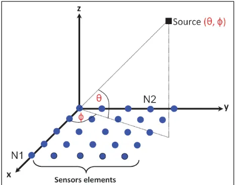
The conventional linear arrays present several limitations, especially to follow — at the same time — variations in direction of the moving signal sources, in both the elevation and azimuth angles. However, a planar array in the 2 dimensions (2D) is necessary to real time radar applications, where various signals can come from the same angle. We described here the popular rectangular array scheme.
Suppose the N1 ×N2 identical elements, uniformly spaced and
positioned in thexoy axes as depicted in Figure 1.
Figure 1. Schematic illustration of a rectangular sensor array.
signals, we can express the total received vector as follows [28]:
X(t) = K
i=1
si(t)Ai+N(t) (1)
where X(t) is the N1 × N2 data matrix, and N(t) is a matrix
representing the received noise vector which can be considered here as Gaussian, spatially white, of null mean andσ2N variance.
The directional vector of the ith signal Ai is the Kronecker product [29] between columns and rows [28]. si(t) is the amplitude of the ith received signal.
For the adaptive beamforming using a conventional LMS algorithm, the adaptive weights are adjusted by the Mean Square Error (MSE) approach, which minimises the error between the output signals of the array, and given by
y(t) =WHX(t) (2)
where W represent the weight vector, (·)H expresses the conjugate transpose. The weight vectorW is given by:
For conventional LMS algorithm, the misadjustment M can be approached by the known formula [30]:
M ≈μN λave (4)
where λave represents the mean of Eigen value of the input autocorrelation matrices (μis the algorithm step size).
We notice that the misadjustment increases linearly with the number of sources array elements, and hence, the reduction of the elements array dimensionality decreases M, which give arise for algorithms with partial adaptability (i.e., the use of sub-arrays concept).
3. CONFIGURATION OF SUBARRAYS
Optimum processing at subarray level seems to have the most advantages for reasons of performance and practical implementation. However, subarray configuration is not a trivial problem in array signal processing. A proper subarray configuration is important to improve the detectability of any given array. The question of how adaptive interference suppression with multifunction phased array radar with subarray beamforming should habitually be considered. The problem of how to arrange the subarray is crucial. Among the various possible subarray configurations, the most efficient and simple architecture is the one which consists in grouping the elements of the array which are directly “followed”, to form what is largely called the “simple subarray”. Nonetheless, the inherent problem of this efficient configuration is the fact that the “phase-centers-subarray” are spaced with several wavelengths [31]. This situation gives place to the known phenomenon of “Grating lobes”.
To circumvent this problem, alternative configuration which can be more adapted to the rectangular array geometry used here is the “row-column precision array” [31]. In this configuration, the resulting number of weights is equal to the number of rows plus the whole number of columns of the array. We use this configuration in our problem formulation because it deals well to the partial adaptivity.
4. SEQUENTIAL BLOCK LEAST MEAN SQUARE (SBLMS) ALGORITHM
adaptivity by row/column precision array gives place to two subsets: One for the row-elements, and another for the column-elements.
To reduce the convergence-time while keeping the possibility of increasing μ, the best way is the use of the block LMS algorithm (BLMS) [33].
Combination of these two algorithms gives place to a newly hybrid algorithm calling here as “SBLMS” (this hybrid algorithm will be analyzed in the next section).
The weight vector of the BLMS algorithm can be given by:
w(k+ 1) =w(k) + 2μB
L X
T(k)e(k) (5)
where L is the block length andμB represent the adaptation step of BLMS algorithm, and
e(k) =d(k)−W(k)HX(k)
is the error vector, and k represents the order of the samples’ block. For SLMS algorithm, the weight vector is given by:
w(k+ 1) =w(k) + 2μXT(k)Iie(k) (6)
whereIi is the matrix-identity used to choose theith set of the weights from theP sets. In this case,kindicates the sample’s iteration. Finally, the weight vector of the resulting algorithm (SBLMS) is given by:
w(k+ 1) =w(k) + 2μB
L X
T(k)Iie(k) (7)
where Ii is the matrix-identity of an appropriate dimension. It represents the sets formed in partial adaptivity. When we adopted the “row-column precision array” configuration, then we obtain two subsets and the matrices-identity will beI1 andI2.
Two important conclusions can then be drawn:
(i) Godavarti shows that the SLMS algorithm converges in the mean if the LMS algorithm converges in the mean [8], and hence, the same conclusion can be extended to the SBLMS algorithm. (ii) By realising the mean of gradient vectors of SBLMS algorithm, the
5. SIMULATION RESULTS
To carry out the cancellation performances and the tracking possibilities of our newly designed SBLMS algorithm — compared to conventional LMS algorithm — various situations and examples were simulated. The goal is to examine the efficiency of algorithms, the conventional LMS and the SBLMS one, in their ability to
(1) Follow angular displacements (D.O.A) of both target and jam-mers,
(2) To preserve the signal coming from the desired direction, and (3) To cancel all contributions of the jammer.
For that, we simulated mobile sources, deviating in a linear way of 10◦ during the number of samples of processing.
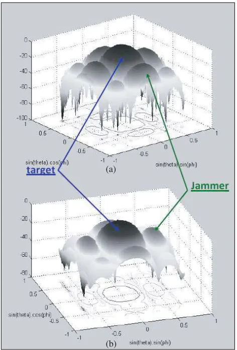
For LMS algorithm, we took a 6×6 rectangular array, the input signal to noise plus interference ratio (SINR) is −20 dB. The input signals of the array are shown in Figures 2(a) and 2(b), respectively.
(a) (b)
(c) (d)
Figure 2(c) shows the error variation between the desired signal and the output of the adaptive array. Thus, we observe that after about sixty samples, the error is clearly minimized. Interestingly, the algorithm could maintain the level of error under the value of 0.05. In Figure 2(d), we show that the LMS algorithm could easily recover the desired signal.
The three dimensional representation of the beam pattern makes it possible to clearly show the change in the output beam pattern after adaptation (See Figure 3).
(a)
(b)
On Figure 3(b), one can note that in the direction of the target energy is maintained largest (see arrows). The representation of the beam pattern in the contour form makes it possible to better see the shift of the main lobe from 0◦ to 10◦ (i.e., 0.18 in the sin(θ)·cos(φ) axes).
We will now remake the same simulations with SBLMS algorithm, by using 1000 samples divided into two (02) blocks. Thus, the number of iteration is 500. The weight vector size in this case is 6 + 6.
According to Figure 4, we note that the desired signal was succefully recovered and the error highly minimized, with a much faster
(a) (b)
Figure 4. The SBLMS algorithm signals. The output (a) and (b) the error signal.
convergence, i.e., in a smaller number of samples than that obtained in the case of the conventional LMS algorithm.
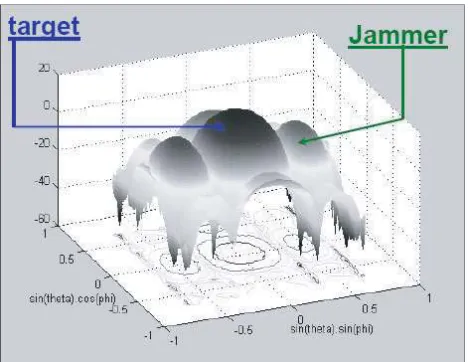
The modification of the beam pattern, after the use of SBLMS algorithm, is carried out by the 3-dimensional representation.
Figure 5 shows that, the beam pattern after adaptation presents a higher level amplitude in the direction of the desired signal compared to that of the array beam pattern before adaptation (Figure 3(a)), whereas in the direction of the jammer, it’s strongly attenuated.
It is worth noting here that the speed of the jammer-displacement and/or the target influence obviously the tracking behavior of the algorithm. A conventional evaluation method of the robustness of algorithms for a given array consists in calculating their output signal to noise plus interference ratio (SINR).
For simulation, we took the same conditions as previously, applied to 8×8 uniform rectangular arrays (URA). The input SINR is−20 dB, in 800 iterations.
Figure 6 clearly shows that for the two algorithms (LMS and SBLMS), the angular shift has increased, as a result of a deterioration of the performances of the adaptive systems, and hence, a reduction of the SINR. In fact, we do note that performances of SBLMS algorithm are definitely better than those of conventional LMS, in particular when the angular shift increases. Thus, for an abrupt displacement of 15◦, the output SINR passed to−1.2 dB for the LMS and approximately to 8 dB for the SBLMS (See Figure 6).
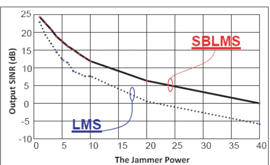
Figure 7. Power jammer influence on the output SINR on: SBLMS (solid curve) and LMS (dash curve).
Finally, we test the effect of the power of jammers on the behaviors in tracking and cancelation of jammers. A comparison between the two algorithms, LMS and SBLMS is then done. As expected, it’s a clear that a comparison between SBLMS algorithm and LMS algorithm gives the advantage to the SBLMS, where Figure 7 shows the degradation of the output SINR of the adaptive array when the power of the jammer increases.
6. CONCLUSION
of this algorithm to achieve the jammers suppressions tasks, and its dominant convergence rate performance compared to that of the conventional LMS.
REFERENCES
1. Ares-Pena, F. J., G. Franceschetti, and J. A. Rodriguez “A simple alternative for beam reconfiguration of array antennas,”Progress In Electromagnetics Research, PIER 88, 227–240, 2008.
2. Zhou, H.-J., B.-H. Sun, J.-F. Li, and Q.-Z. Liu, “Efficient optimization and realization of a shaped-beam planar array for very large array application,” Progress In Electromagnetics Research, PIER 89, 1–10, 2009.
3. Zhang, S., S.-X. Gong, Y. Guan, P.-F. Zhang, and Q. Gong, “A novel iga-edspso hybrid algorithm for the synthesis of sparse arrays,” Progress In Electromagnetics Research, PIER 89, 121– 134, 2009.
4. Wang, Y., G. Liao, Z. Ye, and X. Wang, “Combined beamforming with alamouti coding using double antenna array group for multiuser interference cancellation,”Progress In Electromagnetics Research, PIER 88, 213–226, 2008.
5. Cengiz, Y. and H. Tokat, “Linear antenna array design with use of genetic, memetic and tabu search optimization algorithms,” Progress In Electromagnetics Research C, Vol. 1, 63–72, 2008. 6. Mahanti, G. K., A. Chakrabarty, and S. Das, “Phase-only
and amplitude-phase only synthesis of dual-beam pattern linear antenna arrays using floating-point genetic algorithms,” Progress In Electromagnetics Research, PIER 68, 247–259, 2007.
7. Henin, B. H., A. Z. Elsherbeni, and M. H. Al Sharkawy, “Oblique incidence plane wave scattering from an array of circular dielectric cylinders,”Progress In Electromagnetics Research, PIER 68, 261– 279, 2007.
8. Gozasht, F., G. Dadashzadeh, and S. Nikmhr, “A comprehensive performance study of circular and hexagonal array geometreis in the LMS algorithem for smart antenna applications,”Progress In Electromagnetics Research, PIER 68, 281–296, 2007.
9. Mouhamadou, M., P. Armand, P. Vaudon, and M. Rammal, “Interference supression of the linear antenna arrays controlled by phase with use of SQP algorithm,” Progress In Electromagnetics Research, PIER 59, 251–265, 2006.
phased array systems,” Progress In Electromagnetics Research, PIER 53, 227–237, 2005.
11. Aissa, B., M. Barkat, M. A. Habib, B. Atrouz, and M. C. Yagoub, “An adaptive reduced rank stap selection with staggered PRF, effect of array dimensionality,” Progress In Electromagnetics Research C, Vol. 6, 37–52, 2009.
12. Frost, O. L., “An algorithm for linearly constrained adaptive array processing,”Proc. IEEE, Vol. 60, 926–935, Aug. 1972.
13. KO, C. C., “Power inversion array in a rotating source environment,”IEEE Trans. Aerosp. Electron. Syst., Vol. 16, 155– 762, Nov. 1980.
14. Davies, D. E. N., “Independent angular steering of each zero of the directional pattern of a linear array,”IEEE Trans. Antennas Propagat., Vol. 15, 296–298, 1967.
15. Khanna, R. and B. B. Madan, “Adaptive beamforming using a cascade configuration,” IEEE Trans. Acoust., Speech, Signal Processing, Vol. 31, 940–945, 1983.
16. Compton, R. T., “On the Davies tree for adaptive array processing,” IEEE Trans. Acoust., Speech, Signal Processing, Vol. 33, 1019–1021, 1985.
17. KO, C. C., “Adaptive array processing using the davies beamfonner,” Proc. Inst. Elec. Eng., Vol. 133, Pt. W, 467–473, 1986.
18. Capon, J., R. J. Greenfield, and J. Kolker, “Multidimensional maximumlikelihood processing of a large aperture seismic array,” Proc. IEEE, Vol. 55, No. 2, 192–211, Feb. 1967.
19. Griffths, L. J. and J. W. Jim, “An alternative approach to linearly constrained adaptive beamforming,” IEEE Trans. Antennas Propagat., Vol. 30, No. 1, 27–34, Jan. 1982.
20. Lee, J. C. and C. K. Un, “Performance of transform-domain LMS adaptive digital filters,”IEEE Trans. Acoust., Speech, Signal Processing, Vol. 34, No. 3, 449–510, Jun. 1986.
21. Boroujeny, B. F. and S. Gazor, “Selection of orthonormal transforms for improving the performance of the transform domain normalised LMS algorithm,” IEE Proc-F, Vol. 139, No. 5, 327– 335, Oct. 1992.
22. Frost, O. L., “An algorithm for linearly constraint adaptive array processing,”Proc. IEEE, Vol. 60, No. 8, 926935, Aug. 1972. 23. KO, C. C., “Simple eigenvalue-equalizing preprocessor for
24. Yuen, S. M., “Exact least-squares adaptive beamforming using an orthogonalization network,”IEEE Trans. Aerosp. Electron. Syst., Vol. 27, No. 2, 311–330, Mar. 1991.
25. Haykin, S., A. H. Sayed, J. Zeidler, P. Yee, and P. Wei, “Adaptive tracking of linear time-variant systems by extended RLS algorithms,” IEEE Trans. Signal Processing, Vol. 45, No. 5, 1118–1128, May 1997.
26. Youcef, N. R., “A unified approach to the steady-state and tracking analyses of adaptive filters,” IEEE Trans. Signal Processing, Vol. 49, No. 2, 314–324, Mar. 2001.
27. Douglas, M., “Adaptive filters employing partial updates,”IEEE Trans. Acoust., Speech, Signal Processing, Vol. 44, 209–216, Mar. 1997.
28. Lee, C. C. and J. H. Lee, “Design and analysis of a 2-D eigenspace-based interference canceller,” IEEE Trans. Antennas Propagat., Vol. 47, No. 4, 733–743, Apr. 1999.
29. Graham, A., Kronecker Products and Matrix Calculus with Applications, Halsted Press, John Wiley and Sons, NY, 1981. 30. Widrow, B. and S. D. Stearns, Adaptive Signal Processing,
Prentice-Hall, Englewood Cliffs, NJ, 1985.
31. Chapman, D. J., “Partial adaptivity for the large array,” IEEE Trans. Antennas Propagat., Vol. 24, No. 5, 685–696, Sep. 1976. 32. Godavarti, M., “Antenna arrays in wireless communications,”
Dissertation of Electrical Engineering and Computer Science, University of Queensland, 2001.