A Method for Ice-Thickness Detecting and Ice-Section Imaging
by Using FMCW-SAR Algorithm
Rui Zhao, Yu Tian*, Ling Tong, and Bo Gao
Abstract—Sea ice plays an important role in global climate. Many researches focus on the measurement of the sea ice thickness. In this paper, we present a method for the ice-detecting combining frequency-modulated continuous-wave (FMCW) technology and synthetic aperture radar (SAR) technology. It can provide a good resolution both in the range dimension and the azimuth one. Then a simulation is conducted to verify the accuracy and the feasibility of this algorithm. The physical properties of the sea ice, such as reflection and scatter properties of the ice surface and the transmission characteristic when the electromagnetic wave travels through the ice, are considered in the simulation. The results of the simulation demonstrate that this algorithm has a good performance in ice penetrating.
1. INTRODUCTION
The detection of ice thickness has been a research hotspot [3–6], because sea ice plays an important role in global climate change [1, 2].
For now, the measurements of the ice thickness have been roughly divided into two kinds of measurement. One is remote sensing technology which can measure the ice thickness or the amount of ice for a very large area; however, a lot of statistical computing needs to be done because of poor accuracy. The other is on-site measurement [4, 5] which could provide more accurate data and meet the real-time requirements. Furthermore, it could be used for the calibration of remote sensing data. But most of them focus on the fixed-point ice thickness instead of continuous ice-thickness information along a path. In [16], the professional probing of sub-bottom profiler is based on this way that it detects the ground for many times and records the data, then images the section according to the different measured values corresponding to specific positions. In consequence, the resolution along the detection trace is related to the distance between the measuring points, and it is always poor.
This paper presents a new on-site measurement based on the FMCW-SAR technology which combines the FMCW and SAR algorithms. It can get accurate information of the ice thickness as FMCW radar does. In addition, it can creatively image the ice section with a high resolution in azimuth dimension and provide more abundant information for research.
While few SAR applications can image in the depth dimension, almost all of the studies in correlation with SAR, no matter the traditional SAR [10] or FMCW-SAR [11, 12], focus on the application that will collect the echo from only one surface. The final processed image presents the relative information of a fixed area of the earth’s surface. Besides, the echo is affected by specific physical property of the sea ice, such as reflection factor, refraction factor and loss. With these factors, FMCW-SAR may lose efficacy when the algorithm is used in detecting the sea ice. A ground penetrating radar [17] can image in the depth dimension of the ground, while it is always the pulse pattern SAR (not the FMCW-SAR). In addition, the radar is installed just on the ground or a few centimeters above. Thus it is not the same as ice-thickness detecting by using FMCW-SAR presented in this paper.
Received 18 February 2016, Accepted 7 May 2016, Scheduled 18 May 2016 * Corresponding author: Yu Tian ([email protected]).
Taking the factors mentioned above into account, the primary task of this paper is to verify the feasibility of the detection of the sea ice thickness by using the FMCW-SAR algorithm. This paper discusses the related algorithm (FMCW-SAR) used in this radar system in Section 2. Then a simulation of this radar system and algorithm are discussed in Section 3 and Section 4. The simulation includes the modeling of a transmitting waveform (FMCW), effect of ice physical property, calculating of the echo and data processing of the radar system. At the end of the paper, corresponding results and summaries are given. Because of the restriction of place and equipment in the laboratory, we are not able to conduct the relative field experiments for now. Nevertheless, the disadvantages will be made up in the future work.
2. SPACE GEOMETRIC MODEL AND THEORETICAL ANALYSIS
The radar system is just the FMCW radar system. But, the transmitting and receiving antennas are installed vertically towards the ice. The beam width along the detection trace should be as wide as possible to improve the resolution in this direction. In order to reduce the influence of the scattering echo out of the detection trace, the beam width in the vertical direction of the detection trace should be kept narrow.
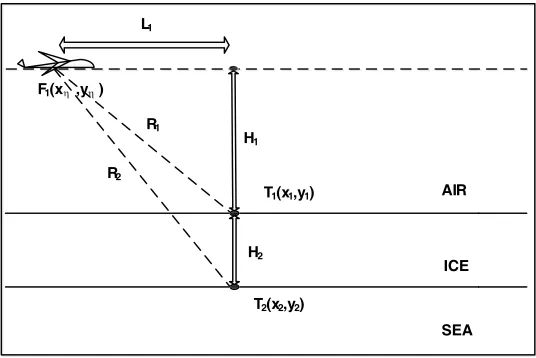
The radar operating model is based on the strip-map SAR model, which performs imaging of a strip on the ground aside the flight trajectory. The space geometric model in this paper is shown in Fig. 1. The radar system is installed on an aircraft. The aircraft flies along a straight line (x-axis) with velocity V at altitude H above the ice. The radar on the plane transmits electromagnetic wave and collects the echo from the targets (T1,T2) at different times. F1,F2,F3,F4,F5 are the locations of the
aircraft at different times.
X
Y
T1(x1,y1) T2(x2,y2)
F1(x3,y3) F2(x4,y4) F3(x5,y5) F4(x6,y6) F5(x7,y7)
AIR
ICE
SEA V(velocity)
Figure 1. The space geometric model.
R1 =
L2
1+H12 (1)
L1 = |xη−x1| (2)
H1 = |yη−y1| (3)
R1 =
|xη −x1|2+|yη−y1|2 (4)
The following is a brief introduction about the FMCW-SAR algorithm under the circumstances of considering only one single target T1 in Fig. 2 and hypothesizing thatT1 is the origin ofxcoordinates.
Define the time of the electromagnetic wave propagation form the radar to targetT1 and then return to
T1(x1,y1)
T2(x2,y2) F1(xη ,yη )
AIR
ICE
SEA H1
H2 R1
R2 L1
Figure 2. The space geometric model at a certain moment.
interval. Then the time used by the plane for traveling along the flight trajectory is defined as slow time (η). We can suppose that the plane is stationary during the fast time (t) because of the relation
ηt (5)
Then x-coordinate (xη) for plane location is
xη =vη (6)
The transmitting signal is
St(t, η) =A0Wr[t]Wa[η−η1]ej(2πf0t+πKrt 2)
(7)
whereA0Wr[t]Wa[η−η1] is a envelop function;Wr[t] andWa[η−η1] are rectangular window functions;
f0 is the carrier frequency;Kr is the frequency sweep rate.
The receiving signal is
Sr(t, η) =A0Wr[t]Wa[η−η1]ej(2πf0(t−τ)+πKr(t−τ) 2)
(8)
whereτ is the delay time. It correlates with the distance (Rη) between the target and radar.
τ = 2Rη
c (9)
The IF signal is obtained after the mixing of the transmitting and receiving signals.
Src(t, η) =AtWr[t−τ]Wa[η]ej2πf0τ−jπKrτ2ej2πKrτt (10) De-chirp principle is used in FMCW radar system to compress range dimension. All it needs is processing signal by frequency transform in fast time dimension.
Src(fr, η) =AtPr
fr−Kr2Rcη
Wa[η]ej2πf02Rηc e−jπKrτ2 (11)
where Pr
fr−Kr2Rcη
is a sinc function. The last part e−jπKrτ2 is redundant and can be offset by
multiplying its penalty function ejπKrτ2 based on different delay times.
Src(fr, η) =AtPr
fr−Kr2Rcη
Wa[η]ej2πf0
2Rη
c (12)
In RD algorithm (one of the SAR algorithms), the range (Rη) is approximated [10]
Rη =
(vη)2+H12 ≈H12+(vη)
2
2H1
(13)
Apply Eq. (13) into Eq. (12),
Src(fr, η) =AtPr
fr−Kr2Rcη
Wa[η]e−j4πf0Hc1e−jπ2v 2
λH1η2 (14)
Frequency transform in slow time dimension is applied [10].
Srcf(fr, fη) =F F Tη(Src) =AtPr
fr−Kr2Rcη
Wa[fη]e−j4πf0Hc1ejπ fη2
Ka (15)
After the Range Cell Migration Correction [10], compression in fη dimension is to remove nonlinear phase by multiplying the compression function
Haz(fη) =e−jπ
fη2
Ka (16)
Then the final function is obtained after IFFT infη dimension.
Srcf(fr, η) =AtPr
fr−Kr2Hc1
Pa[η]e−j4πf0
H1
c (17)
wherePa[η] is a sinc function.
We can see that infr dimension the signal is compressed at the pointKr2H1
c which contains range
information. In η dimension, the signal is compressed at point 0. It is the exact location of T1. If the
target is a specific point, it will be compressed at the position where Doppler frequency is 0 [10]. So the above algorithm can realize point compression. In ice detection application, we can get ice thickness information as long as we compress the target points on the top and bottom of sea ice in its actual position.
3. DESIGN FOR SIMULATION
The above algorithm is deduced in ideal situation. In practice, the backscattering coefficient, reflection coefficient, loss in sea ice and other factors should be considered. In order to examine whether the algorithm can be used in the detection of sea ice, a simulation including these factors is designed.
modulating
signal VCO
Signal generator BPF Coupler AMP
Antenna
Antenna LNA BPF MIXer
Transmitter
Receiver IF signal
processing
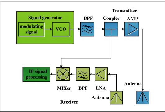
Figure 3 shows a hardware sketch map of the FMCW radar system. The transmitting signal is generated by VCO and transmitted to the target through transmitting antenna. After the signal is reflected and scattered from the top and bottom surfaces of the sea ice, the echo will be collected by the receiving antenna. Then IF signal is obtained for processing by mixing the receiving signal and the transmitting signal obtained from the power divider. So the simulation concentrates on the following parts: modeling the transmitting and receiving signals, reflection and backscattering term, the damping through sea ice and the generation of IF signal.
3.1. Geometric Model of Bottom Surface Echo
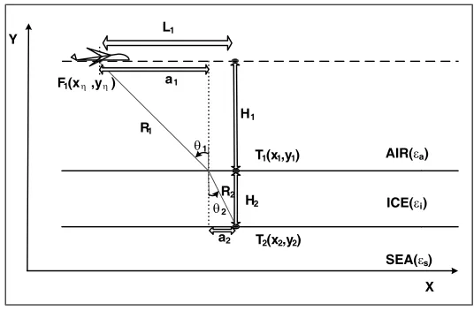
The modeling of transmitting and receiving signal is based on the algorithm introduced in Section 2. Equation (7) shows mathematical expression of the original signal. The mathematical expression of the receiving signal is in Eq. (8). The delay time τ is relative to the distance between the radar and one target. For the point targets on the top surface, the distance is calculated as in Eq. (1). However, for those on the bottom surface, we should consider the influence of refraction phenomenon. Fig. 4 shows the space geometric model about the point target on bottom surfaces.
X Y
T1(x1,y1)
T2(x2,y2) F1(xη ,yη )
AIR(εa)
ICE(εi)
SEA(εs) H1
H2 R1
R2 L1
θ1
θ2 a1
a2
Figure 4. space geometric model of echo from bottom surface.
As shown in Fig. 4, at a certain moment, L1, H1 and H2 are known. The dielectric constants
of air, ice and sea are εa, εi, εs, respectively. What we need is the distance of electromagnetic wave propagation path from the radar (F1) to a target on bottom surface (T2) .
Rη =R1+R2 (18)
On the top surface, considering the reflection phenomenon
n1sinθ1 =n2sinθ2 (19)
wheren1 and n2 are the refractive index of two media.
sinθ1 = Ra1 1
(20)
sinθ2 = a2
R2
(21)
a1+a2=L1 (22)
R1 =
a2
1+H12 (23)
R2 =
a2
2+H22 (24)
3.2. The Damping Lost in Sea Ice
The component of sea ice is very complex. The dielectric constant varies with the difference in temperature, salinity and other factors, and it is a complex number. The loss relates to its imaginary part and mainly affects the echo energy and then affects the detectability of the radar.
Assuming that the electromagnetic wave will transmit along z direction in a medium, the electromagnetic wave transmission function is
S=Ae−γz (25)
where z is the transmitting distance along z direction, and γ is the propagation constant and can be calculated by the equation
γ =jω√μiεi (26)
where μi is the permeability of sea ice and εi the dielectric constant. Then we know that γ is still a complex number. Assume that
γ =α+jβ (27)
Then,
S=Ae−aze−jβz (28)
From Eq. (28), the first part e−az presents that the amplitude exponentially decays with the increase of distancez. So it is called decay factor.
3.3. Reflection Model
As shown in Fig. 1, when the plane flies just on the point target (F3), the incident angle of the
transmitting signal is 0, and reflection model is more suitable. Reflection model is more suitable [13].
AIR(εa)
ICE(εi)
SEA(εs)
St Sr1
Sit Sir
Sr2
Γ Γ
Γ Z2
Z1
Z3
ai ia
is
Figure 5. Reflection model of radar signal when it is irradiated on ice surface.
Figure 5 shows the reflection model of radar signal when it is irradiated on ice surface. St is the incident wave power, and Sr1 and Sr2 are the reflection signal powers of the top and bottom surfaces.
Reflection and refraction phenomenon will occur at the points Z1, Z2, Z3 according to the Fresnel
formula. At point Z1.
Sr1 = Γ2aiSt (29)
Sit = 1−Γ2aiSt (30)
Then it is the same at points Z2 andZ3. So
Sr2 =
If we define that
Γ2r1= Γ2ai (32)
Γ2r2 =1−Γ2iaΓ2is1−Γ2ai (33) Then
Sr1 = Γ2r1St (34)
Sr2 = Γ2r2St (35)
The power of the signal collected by receiving antenna can be calculated by the formula [13]
Pr = Ptλ
2G2|Γ|2
(4π)2(2R)2 (36)
where Pt is the transmitting power of radar, G the gain of transmitting or receiving antennas, R the distance from the radar to the top surface of sea ice, λthe wave length of the transmit signal and Γ the reflection coefficient. Γr1 and Γr2 are obtained in the case that the surfaces are perfectly planar.
When the surfaces are rough with the value of rms height, a parameter for measuring the roughness of the surface is σh. The formula is as follow [14]
Γ = Γre−4K2σh2 (37)
where Γr is the reflection coefficient calculated in an ideal situation, and K is the wave number. It should be mentioned that approximation is used to make the simulation faster and make it concentrate on the impact of main factors (reflection, refraction, back scattering). The values of the wave number
K and wave length lambda are the factors when the frequency is the center frequency of the bandwidth. Although it will cause some distortion, the approximation is tolerable for the purpose of demonstrating the efficiency of the algorithm when it is used in detecting ice thickness. Because it affects only the envelop function of the receiving signal, the change of the envelop is much slower relative to the change of phrase. Besides, the received signal will be windowed before processed by the algorithm, which can reduce the impact caused by the approximation. [7, 8, 18, 19] also use the narrow-band communication technology and make the same approximation when they exposit the theory or design the relative simulation.
3.4. Back Scattering Model
In addition to the conditions mentioned above, when the angle of incidence is not zero, the receiving signal is characterized by scattering term because of roughness of the sea ice surfaces.
The classic Kirchhoff model is used in this paper [13].
σp(θ) = |R(0)|
2
2σ2
scos4θ
e
−tan2θ
2σs2
(38)
whereσs is the surface slope which is also a factor for measuring the roughness of the surface. R(0) is the Fresnel reflection coefficient andθ the angle of incidence.
3.5. Parameters for Simulation
Table 1 shows the radar parameters used in this simulation.
The physical information of sea ice refers to [13] and [15]. The data used in [13] is obtained from a roughness measurement experiment conducted in Antarctica during September 2003. [15] uses the data collected in the southern Beaufort Sea in the winter of 2008 from the research icebreaker CCGS Amundsen as part of the Circumpolar Flow Lead (CFL) system study.
Table 1. Radar parameter.
start frequency(fstart) 8Ghz stop frequency(fstop) 12 Ghz
Band width(B) 4 Ghz pulse repetition time(Tm) 0.1 ms
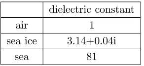
Table 2. Physical parameters of air,sea ice and sea.
dielectric constant
air 1
sea ice 3.14+0.04i
sea 81
Table 3. Roughness factors of top and bottom surfaces.
RMS height (m) correlation length (m)
top surface 0.01 0.1
bottom surface 0.01 0.1
Table 4. Two schemes of chosen point targets.
Scheme 1 Scheme 2
top H1(0,2995) H1(−50,2995) H2(−20,2985) H3(0,2995) H4(20,2985) H5(50,2995)
bottom H2(0,3005) H6(−50,3015) H7(−20,3015) H8(0,3010) H9(20,3015) H10(50,3010)
4. SIMULATION RESULTS AND DISCUSSIONS
In order to verify the correctness of the algorithm used in the detection of the ice thickness, coordinate system is established as shown in Fig. 1. Two schemes of chosen point targets are displayed in Table 4. The damping loss in the ice which only affects the amount of energy is ignored temporarily.
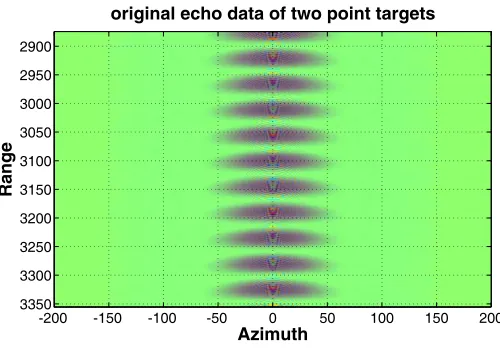
The consequence without loss is shown in Fig. 6–Fig. 11.
Figures. 6, 7 and 8 show that for two point targets from top and bottom surfaces respectively, the algorithm can detect them even though it has a little defocusing that may lead to performance degradation of resolution.
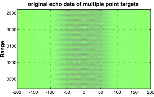
Figures 9, 10 and 11 are the results of the multiple point targets simulation. As shown above, the FMCW-SAR algorithm puts up a good performance in detecting the point targets. Fig. 11 is the comparison between the processed focus points and the original ones which we set for the simulation. The two green lines in the figure are the ligature of the original point targets. The results demonstrate that the algorithm does very well in the inversion of the positions of the different point targets on the top and bottom ice surfaces.
In summary, the simulation results prove that the algorithm is feasible in detecting the ice thickness. When considering the loss in ice, the consequences of the first scheme is shown in Fig. 12.
Azimuth
Range
original echo data of two point targets
-200 -150 -100 -50 0 50 100 150 200
2900
2950
3000
3050
3100
3150
3200
3250
3300
3350
Figure 6. Original echo data of two point targets.
Azimuth
Range
two points image after processed
-20 -15 -10 -5 0 5 10 15 20
2970
2980
2990
3000
3010
3020
3030
Figure 7. Two points image after processed.
Figure 8. Two points squint image after processed.
damping or the thickness of the ice.
Range
original echo data of multiple point targets
-200 -150 -100 -50 0 50 100 150 200
2900
3000
3100
3200
3300
Figure 9. Original echo data of multiple point targets.
Azimuth
Range
multiple point targets image after processed
-60 -40 -20 0 20 40 60 2960
2970
2980
2990
3000
3010
3020
3030
3040
Figure 10. Multiple point targets image after processed.
Azimuth
Range
point targets image
-60 -40 -20 0 20 40 60
2960
2970
2980
2990
3000
3010
3020
3030
3040
Figure 11. Comparison between processed focus points and original ones.
the dielectric constant of the sea ice is 3.14 + 0.04i, and the wave length is 0.06 m. The simulation method is mentioned in Section 3.2.
Azimuth
Range
two point targets image with loss
-20 -15 -10 -5 0 5 10 15 20
2970
2980
2990
3000
3010
3020
3030
Figure 12. Two point image with loss.
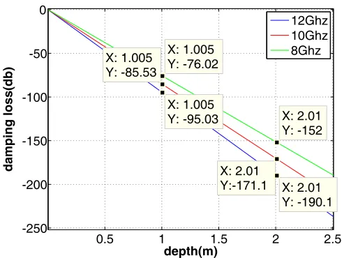
0.5 1 1.5 2 2.5 -250
-200 -150 -100 -50 0
X: 2.01 Y: -152
depth(m)
damping loss(db) X: 2.01
Y:-171.1 X: 2.01 Y: -190.1 X: 1.005
Y: -95.03 X: 1.005
Y: -85.53
X: 1.005 Y: -76.02
12Ghz 10Ghz 8Ghz
Figure 13. Amplitude attenuation of 3 different frequency signals versus depth of sea ice.
signals are more than 76 db, and the values increase rapidly as the depth of the sea ice increases. So it is not suitable for detecting the ice which is too thick. Of course, it could only be used as a reference. The loss will change a lot under different actual detection environments.
5. SUMMARY AND FUTURE WORK
From the above introduction, the consequences of the simulations can illustrate the feasibility of the algorithm. Nevertheless, more works need to be done in the future due to the incompletion of the algorithm.
ACKNOWLEDGMENT
This work is supported by the National Natural Science Foundation of China(Grant No. 61201006).
REFERENCES
1. Etkins, R. and E. S. Epstein, “The rise of global mean sea level as an indication of climate change,”
Science, Vol. 215, 287–289, 15 Jan. 1982.
2. ACIA,Arctic Climate Impact Assessment, Cambridge University Press, New York City, New York, 1042, 2005.
3. Gogineni, S., Z. Wang, J. B. Yan, et al., “Wideband radar for ice sheet sounding and imaging,”
General Assembly and Scientific Symposium (URSI GASS), 2014 XXXIth URSI. IEEE, 1, 2014.
4. Dall, J., A. Kusk, S. S. Kristensen, et al., “P-band radar ice sounding in Antarctica,” Geoscience
and Remote Sensing Symposium (IGARSS), 2012 IEEE International. IEEE, 1561–1564, 2012.
5. Gogineni, S., J. B. Yan, D. Gomez, et al., “Ultra-wideband radars for remote sensing of snow and ice,”Microwave and RF Conference, 2013 IEEE MTT-S International, IEEE, 1–4, 2013.
6. Wu, C., X. Zhang, J. Shi, et al., “Radar signal simulation on investigation of subsurface structure by radar ice depth sounder,”Geoscience and Remote Sensing Symposium (IGARSS), 2014 IEEE International, IEEE, 4848–4851, 2014.
7. Han, H. and H. Lee, “Radar backscattering of lake ice during freezing and thawing stages estimated by ground-based scatterometer experiment and inversion from genetic algorithm,”IEEE Transactions on Geoscience and Remote Sensing, Vol. 51, No. 5, 3089–3096, 2013.
8. Dagdeviren, B., K. Y. Kapusuz, and A. Kara, “A modular FMCW radar RF front end design: Simulation and implementation,”Signal Processing and Communications Applications Conference (SIU), 2014 22nd. IEEE, 1762–1765, 2014.
9. Kanagaratnam, P., S. Gogineni, N. Gundestrup, and L. Larsen, “High-resolution radar mapping of internal layers at the North Greenland Ice Core Project,” Journal of Geophysical Research, Vol. 106, No. D24, 33,799–33,812, 2001.
10. Cumming, I. G. and F. H. Wong,Digital Processing of Synthetic Aperture Radar Data: Algorithms and Implementation, Artech House, 2005.
11. Luo, Y., H. Song, R. Wang, et al., “Signal processing of Arc FMCW SAR,”IEEE 2013 Asia-Pacific Conference on Synthetic Aperture Radar (APSAR), 412–415, 2013.
12. Smith, R. L., Micro Synthetic Aperture Radar Using FM/CW Technology, Brigham Young University, 2002.
13. Krishnan, S., Modeling and Simulation Analysis of An FMCW Radar for Measuring Snow Thickness, University of Kansas, 2000.
14. Ulaby, F. T., R. K. Moore, and A. K. Fung, Microwave Remote Sensing: Active and Passive, Vol. 2, Artech House, Norwood, MA, 1986.
15. Komarov, A. S., D. Isleifson, D. G. Barber, et al., “Modeling and measurement of C-band radar backscatter from snow-covered first-year sea ice,” IEEE Transactions on Geoscience and Remote Sensing, Vol. 53, No. 7, 4063–4078, 2015.
16. Cui, S. G., H. S. Liu, H. Yi, and J.-L. Wu, “Surface-related multiple elimination on high-resolution geopulse profile,”China Ocean Engineering, No. 2, 331–339, 2008.
17. Kikuta, T. and H. Tanaka, “Ground probing radar system,” IEEE Aerospace and Electronic Systems Magazine, Vol. 5, No. 6, 23–26, 1990.
18. Nielsen, U. and J. Dall, “Direction-of-Arrival estimation for radar ice sounding surface clutter suppression,” IEEE Transactions on Geoscience and Remote Sensing, Vol. 53, No. 9, 5170–5179, 2015.