Rectangular Wave Beam Based GO/PO Method for RCS Simulation
of Complex Target
Wang-Qiang Jiang1, *, Min Zhang1, Ding Nie1, and Yong-Chang Jiao2
Abstract—The rectangular wave beams-based geometrical optics (GO) and physical optics (PO) hybrid method is applied to the radar cross section (RCS) simulation of complex target. In the implementation process, the incident wave beam is divided into plenty of regular rectangular wave beams. The RCS of target is subsequently harvested from the sum of the contributions from rectangular wave beams. And Open Graphics Library (OpenGL) is used to accelerate ray tracing for the GO/PO method. Here, each pixel corresponds to a rectangular wave beam, which improves the defect that the pixel number should be larger than the patch number on the model and the efficiency in the general OpenGL based GO/PO method. In addition, the patch size in the presented method can be arbitrary as long as the model is described accurately with these patches. The simulation results prove this point and show that the proposed rectangular wave beam-based GO/PO method is feasible and can keep a high calculation accuracy and efficiency with a low pixel number.
1. INTRODUCTION
Many methods allow the calculation of electromagnetic (EM) scattering from the target, such as the method of moments (MoM) [1], finite element method (FEM) [2], geometrical optics (GO) and physical optics (PO) method [3–7]. To improve the accuracy, some researchers adjusted the beam shape [8, 9]. Multiple scattering is also considered to improve the accuracy, such as the shooting and bouncing ray (SBR) technique [10–12] and GO/PO method [13, 14]. The GO/PO hybrid method is usually used to calculate the EM scattering of large targets. Knott [4] used physical optics for single reflections and the combination method for double reflections when calculating radar cross section (RCS) of dihedral coroner reflections. For the SBR and GO/PO methods, determining whether the patch is hit by the EM ray is a time-consuming operation. Therefore, many acceleration techniques for ray tracing have been proposed to reduce computation time. Sundarajan and Niamat [15] used the ray-box intersection algorithm to efficiently determine whether rays hit or miss the bounding box of the target. Jin et al. [16] used octree to reduce the number of ray-patch intersection tests. Tao et al. [10] used kd-tree to reduce the ray tracing time in SBR method. They also used the parallel calculating ability of Graphics Processing Unit (GPU) to accelerate the ray tracing process [11]. Wei et al. [13] used the parallel calculating ability of GPU to reduce the ray tracing time in GO/PO method. Rius et al. [17] proposed the graphical electromagnetic computing method to improve the efficiency of calculating the first-order scattered fields. Fan and Guo [14] employed Open Graphics Library (OpenGL) based GO/PO method to make the ray tracing an easy and efficient work. However, the patch missing problem was not discussed when pixel matrix size is small.
For SBR method, it is required that the density of ray tubes on the virtual aperture perpendicular to the direction of the incident field propagation should be greater than about ten rays per wavelength
Received 24 October 2016, Accepted 27 December 2016, Scheduled 13 January 2017 * Corresponding author: Wang-Qiang Jiang ([email protected]).
in view of the convergence of results [11]. Thus, when EM wave frequency gets higher, the large number of ray tubes will predictably lead to time-consuming calculation of target RCS. For the GO/PO method, the scattered field is the sum of the scattered fields excited by the incident wave and the multi-reflection wave. The EM field scattered from the target is considered to be the sum of the fields scattered from patches on the target model. For the general OpenGL based GO/PO method, the number of ray tubes, which equals pixel number, has nothing to do with wavelength. It demands the pixel number to be larger than the patch number. However, when pixel number is large, tracing reflected rays is a time-consuming process.
Reducing the pixel number directly ensures high calculation efficiency. Thus, the method based on the pixel number is developed. Each pixel corresponds to a small regular rectangular wave beam. The total EM field scattered from target is the sum of scattered fields caused by the small regular rectangular wave beams rather than fields scattered from patches. The calculation accuracy depends on the number of small regular rectangular wave beams in this method. When the small wave beam is designed as a regular rectangle, the projection region on the surface of target is easy to calculate, and the reflection beam becomes convenient to determine.
In the present paper, rectangular wave beams are introduced, and the EM scattered field of rectangular wave beam is derived from the PO field. OpenGL is utilized to trace rectangular wave beams, and the RCS of target with different number of pixels is compared to evaluate the accuracy of the proposed method. EM scattering properties of large complex targets are also calculated with different patch numbers.
2. EM SCATTERED FIELD OF RECTANGULAR WAVE BEAM
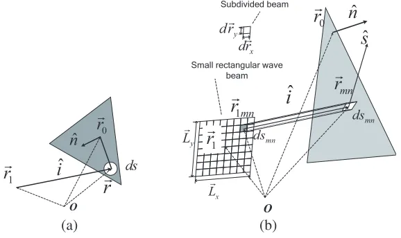
In Figure 1(a), symbol O is the origin point, r1 an arbitrary given point along the center line of the
wave beam, ˆithe unit vector of irradiation direction,r0 an arbitrary, but fixed point on the patch, and
ˆ
nthe unit normal vector. The hit pointr is obtained according to the equation below
r=r1+αˆi (1)
where the coefficient α is expressed as
α=−(r1−r0)·ˆn
ˆi·ˆn (2)
The expression of the square root of RCS√σ is obtained according to [13]
√
σ=i√k π
s
ˆ
er·
ˆ
s×
ˆ
n׈hi
eikr·(ˆi−sˆ)ds (3)
where the ˆsis the unit vector in the direction of propagation of the reflected field, k the wave-number, ˆ
hi the unit vector in the direction of the magnetic incident field, and ˆer the unit vector along the electric
polarization of a far-field receiver.
Figure 1(b) shows one small rectangular wave beam. Its cross section is rectangular with sides of
Lx and Ly. To obtain the EM scattered field of this beam, it is subdivided into 2M×2N rectangular
wave beams, which correspond to a pixel matrix of 2M ×2N. These subdivided beams have sides of
|drx| =|Lx|/(2M) and |dry|= |Ly|/(2N). Position r1 is at the centre of the rectangular wave beam,
and r1mn is the centre position of the (m, n)th subdivided beam with a cross-sectional area dsmn. Its
projection onto the patch surface is dsmn, and the subdivided beam hits the position rmn. According
to Eq. (3), the square root of RCS√σmn of the subdivided beam can be approximated as
√
σmn =i k
√
πˆer·
ˆ
s×
ˆ
n׈hi
eikrmn·(ˆi−ˆs)ds
mn =i
k
√
πeˆr·
ˆ
s×
ˆ
n׈hi
eik(r1mn+αˆi)·(ˆi−ˆs)ds
mn (4)
wherer1mn and α can be expressed as below if the subdivided beams have the same size.
r1mn = (r1+ 0.5drx+ 0.5dry) + (mdrx+ndry) =rc+ (mdrx+ndry)
rc = (r1+ 0.5drx+ 0.5dry)
ˆ n
r
r
0r
r
1r
r
Oˆ
i
dsˆ
n
mnr
r
0r
r
Oˆ
i
mn ds 1mnr
r
x Lr y Lrˆ
s
1r
r
dsmn y drrx drr Subdivided beam
Small rectangular wave beam
(a) (b)
Figure 1. Schematic diagram of (a) hit point, (b) one small rectangular wave beam.
α =
−[(r1+0.5drx+0.5dry)−r0]·nˆ
ˆi·nˆ
+ −(mdrx+ndry)·nˆ ˆi·nˆ
=αc+ −
(mdrx+ndry)·nˆ
ˆi·nˆ
αc =
−[(r1+ 0.5drx+ 0.5dry)−r0]·nˆ
ˆi·nˆ
(6)
Thus, Eq. (4) can be rewritten as
√
σmn = i k
√
πeˆr·
ˆ
s×
ˆ
n׈hi
eik
rc+(mdrx+ndry)+ αc−(mdrx+ˆi·nndˆ ry)·ˆn
ˆi
·(ˆi−sˆ)
dsmn
= i√k πeˆr·
ˆ
s×
ˆ
n׈hi
eik(rc+αcˆi)·(ˆi−sˆ)·eik
(mdrx+ndry)+ −(mdrxˆ+i·nndˆ ry)·nˆ
ˆi
·(ˆi−ˆs)
dsmn (7)
If all subdivided beams of the small rectangular wave beam hit the same patch, the square root of RCS √σ of the small rectangular wave beam is.
√
σ =
m=M−1
m=−M
n=N−1
n=−N i√k
πeˆr·
ˆ
s×
ˆ
n׈hi
eik(rc+αcˆi)·(ˆi−ˆs)·eik
(mdrx+ndry)+ −(mdrxˆ+i·ndnˆ ry)·nˆ
ˆi
·(ˆi−ˆs)
dsmn(8a)
=i√k πˆer·
ˆ
s×
ˆ
n׈hi
eik(rc+αcˆi)·(ˆi−ˆs)·G
ˆi,nˆ,Lx, Lyds
mn (8b)
G
ˆi,nˆ,Lx, Ly= − 2 sin
ς
ˆi,nˆ,s, ˆ Lx
1−ei·ς(ˆi,nˆ,s,ˆLx)/M ·
−2 sin
ς
ˆi,nˆ,s, ˆ Ly
1−ei·ς(ˆi,nˆ,s,ˆLy)/N
(8c)
ς
ˆi
,nˆ,s, ˆ L0
=k L0 2 − L0
2 ·nˆ
ˆi·nˆ ˆi
·ˆi−sˆ (8d)
The area dsmn is given by dsmn = ds|ˆi·mnn|ˆ = 2M·2SN·|ˆi·ˆn|, where S is the cross-sectional area of the
small rectangular wave beam. When M → ∞ and N → ∞, rc becomes the centre position r1 of the
rectangular wave beam. And the result of Eq. (8a) is
√
σ =i√4k πˆer·
ˆ
s×
ˆ
n×hˆi
eik(rc+αcˆi)·(ˆi−ˆs)·F
ˆi,n, ˆ Lx, Ly·S (9a)
F
ˆi,n, ˆ Lx, Ly= 1 4sinc
ς
ˆ
n
1
ˆ
r
i
ˆ
i
1
( cr)
r rr r
2 ˆ
r
i
1 ˆr
n
1 ( 2)
r cr
rr rr
x
Lr
y
Lr
c
r
r
2
xr
Lr
2
yr
Lr
1
xr Lr
1
yr
Lr
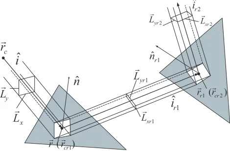
Figure 2. Schematic diagram of reflection beam.
According to Eq. (9), the RCS result of one incident rectangular wave beam can be calculated with parameters, such as ac, source centre position rc of wave beam, irradiation direction ˆi, normal vector
ˆ
n of the irradiated patch, and edge vectors Lx and Ly of wave beam cross section. Parameter ac can
be obtained according to Eq. (2) where r1 is replaced by rc. Because the rectangular wave beam is
assumed to hit on a flat patch, the reflected wave beam is still rectangular. Thus, the RCS result of reflected wave beam can be calculated with the same principle. For example, to calculate the result of the first reflected wave beam, the parameters (ac,rc, ˆi, ˆn,Lx, Ly) should be replaced by the reflected
ray related parameters (acr1,rcr1, ˆir1, ˆnr1,Lxr1,Lyr1). As shown in Figure 2, parameterrcr1 is replaced
by the hit pointr which can be obtained with parameters (rc, ac, ˆi) according to Eq. (1). ˆir1 is the
direction of the first reflected wave beam. ˆnr1 is the normal vector of the patch hit by the first reflection
wave beam. Parameter acr1 is obtained according to Eq. (2) with parameters rcr1, ˆir1, and ˆnr1. Lxr1
and Lyr1 are the edge vectors of the first reflected wave beam. Thus, the square root of RCS, √
σw, of
the rectangular wave beam with multiple reflections can be written as
√
σw = i
4k
√
πˆer·
ˆ
s×
ˆ
n×hˆi
eik(rc+αcˆi)·(ˆi−ˆs)·F
ˆi,n, ˆ Lx, Ly·S
+i√4k πeˆr·
ˆ
s×
ˆ
nr1׈hir1
eik(rcr1+αcr1ˆir1)·(ˆir1−ˆs)·Fˆir1,nˆr1, Lxr1, Lyr1·S
+i√4k πeˆr·
ˆ
s×
ˆ
nr2׈hir2
eik(rcr2+αcr2ˆir2)·(ˆir2−ˆs)·F
ˆi
r2,nˆr2, Lxr2, Lyr2
·S
+. . . (10)
where symbol ˆirn is the nth reflection beam, and ˆnrn is the normal vector of the patch hit by thenth
reflection beam with sides of|Lxrn|and|Lyrn|.
Figure 3 shows that the incident wave beam is divided into many small regular rectangular wave beams. The incident wave beam should be large enough to illuminate the whole target. Its cross section is rectangular with edge vectors Wx and Wy. Then, the edge vectors Lx and Ly of the small regular
rectangular wave beams can be set as Wx/Nx and Wy/Ny, respectively. Nx and Ny are numbers of
small regular rectangular wave beams along the directions ofWx and Wy, respectively. The gray wave
beam misses the target and has a contribution value of zero. The red one, such as thepth rectangular wave beam that hit the target has a contribution value of√σwp, and its contribution can be calculated by Eq. (10). Thus, the square root of RCS for the target is written as
√
σt= p=P
p=1 √
σwp (11)
ˆ
i
x
W
r
/
x x x
Lr Wr N
y
W
r
/
y y y
Lr
=
Wr N=
Figure 3. Incident rectangular wave beam.
3. OPENGL-BASED RAY TRACING
Figure 4 shows a cylinder target projected on the screen. The eye point is a reference point indicating the center of the screen. The process of the EM wave illuminating the target can be treated as the process that human stands in the eye point and observes the target along the viewing direction which is the same as the direction of the incident field propagation ˆi. And the visible patches are those illuminated by EM wave. Functions of OpenGL, such as glViewport, glOrtho and gluLookAt, are used to project the illuminated part on the screen, and the image is generated. The image is treated as a pixel matrix, and each pixel corresponds to a small rectangular wave beam. Given that the eye point and view direction are known, vectors r1 and ˆi for each pixel can be calculated according to the pixel
position. If the patch number (patch ID) is obtained using pixel information, the normal vector ˆnand positionr0 is also obtained according to patch number. Then, the corresponding RCS for the incident
wave is calculated. The RCS for the reflection wave can be calculated using the same method when the eye point and viewing direction are replaced byrand ˆir1 in Figure 2, respectively.
ˆ
i
Figure 4. Target projected in the screen.
screen, and the ID of illuminated patches can be calculated by using the inverse operation of Eq. (12).⎧
⎪ ⎪ ⎪ ⎪ ⎪ ⎪ ⎪ ⎨ ⎪ ⎪ ⎪ ⎪ ⎪ ⎪ ⎪ ⎩
B =int
ID
256×256
G=int
ID−B×256×256 256
R =int
ID−B×256×256−G×256 256
(12)
The patch ID illuminated by the reflection wave beam can be obtained by using the same method. The observing point and view direction are replaced by positionrand reflection direction ˆir1(Figure 2),
respectively.
For some complex situations, the scattered fields of some patches are ineffective. They cannot be received by the receiver in the direction ˆs. To search the effective patches, the position of the receiver is set as the eye point, and the minus direction of ˆs is set as the viewing direction. Then the effective patches can be found and marked with the method of determining patches illuminated by the incident wave. The effective patches have the effective RCS.
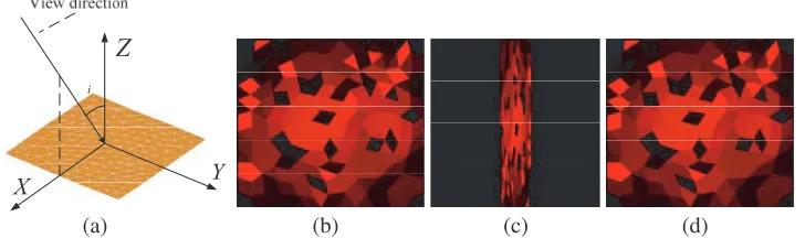
To make full use of the pixel matrix, the display range needs to be adjusted. Figure 5 presents the images of a square plane with different view directions θi. When the view direction θi equals 0◦, the
image of patches covers the whole screen, see Figure 5(b). If utilizing the same display range, the image of patches only covers part of the screen, and the remaining part, where the color is black, is unused, see Figure 5(c). Obviously, the fewer the pixels are used to calculate the EM scattered field, the larger the error occurs. Thus, the display range is changed with the view direction to keep the image of target model covering the pixel matrix as many as possible. Figure 5(d) shows the image with suitable display range, and the pixels of the screen are all effective when the view directionθi equals 80◦.
i
Y
X
Z
(a) (b) (c) (d)
Figure 5. (a) Square plane model, Images with incident angle of (b)θi = 0, (c)θi= 80 with unchanged
display rang, (d) θi= 80 with suitable display range.
For the general method which only considers the scattered field of patches hit by the rays [14], if the size of pixel matrix isM×N and the number of illuminated patches larger thanM×N, some patches are missing. The EM field scattered from target is the sum of fields scattered from patches, and the error will increase with a lower pixel number, as shown in Figure 6. The plane model, illuminated by the incident wave with direction ˆi, is composed of 32 triangular patches. The general method was used on the 4×4 pixel matrix, and only 16 triangular patches were identified, leaving the other 16 patches missing (Figure 6(a)). A serious error will be caused obviously. If the rectangular wave beams-based method is applied, each pixel corresponds to a small rectangular wave beam with a quadrilateral area projected on the plane model (Figure 6(b)). For quadrilateral areas completely covering the whole plane model, the rectangular wave beams-based method has higher accuracy with low pixel number than the general method.
4. NUMERICAL RESULTS
Pixel matrix
Plane model
Pixel matrix
Plane model
Small rectangular wave beam
i
^
i
^
(a) (b)
Figure 6. Situation of low pixels for (a) general method, (b) proposed method.
0 10 20 30 40 50 60 70 80 90 -80
-70 -60 -50 -40 -30 -20 -10 0 10 20 30 40 50
RC
S (
d
Bsm
)
Incident angle i (degree)
Back scattering RCS of square plane
Theory value of PO method Unchanged display range suitable display range
i
X Z
ˆ
i
0 10 20 30 40 50 60 70 80 90 -80
-70 -60 -50 -40 -30 -20 -10 0 10 20 30 40 50
RCS
(
d
Bsm)
Incident angle i (degree)
Back scattering RCS of square plane
General method 50*50 pixels General method 10*10 pixels Proposed method 50*50 pixels Proposed method 10*10 pixels
i
X Z
ˆ
i
θ θ
θ θ
(a) (b)
Figure 7. Back scattering RCS of square plane at 10 GHz with (a) different display ranges, (b) different pixel matrices.
and the black line is the theory value of PO method which only considers the contribution value of the incident wave [13]. The square plane does not undergo multiple reflections, and all its patches are illuminated by incident wave. Because the proposed method is derived from GO/PO method, the theory value in Figure 7(a) is calculated by the general PO method to discuss the influence of display range. As predicted in Figure 5, the results calculated with unchanged display range deviate from the theory value, and the results calculated with suitable display range, which varies with the direction of the incident field propagation θi, fit the theory value well. Thus, it is necessary to adjust the display
range to make full use of pixels on the screen. Otherwise, the error will occur because fewer pixels are used. The results calculated in Figure 7(a) are all with suitable ranges.
;
< =
P
P P
i
^45o
l
θ
(a)
(b) (c) (d)
Figure 8. (a) Trihedral corner reflector model, (b) patches illuminated by incident wave beam, (c) patches illuminated by first reflection wave beams, (d) patches illuminated by second reflection wave beams. (100×100 pixels).
0 10 20 30 40 50 60 70 80 90 0
5 10 15 20 25 30 35 40
Back scattering RCS of trihedral corner reflector
Incident angle i (degree)
RCS
(dB
sm
)
Proposed method MLFMM General method
0 10 20 30 40 50 60 70 80 90 0
5 10 15 20 25 30 35 40
Back scattering RCS of trihedral corner reflector
RC
S (dBsm)
Incident angle i (degree) Size of pixels matrix
100*100 50*50 20*20 10*10 4*4
θ θ
(a) (b)
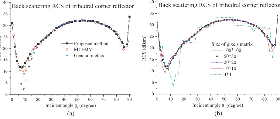
Figure 9. VV-polarization RCS of trihedral corner reflector with (a) different methods, (b) different sizes of pixel matrix. (6 GHz).
A trihedral corner reflector is used to test the accuracy of the improved GO/PO method. Figure 8(a) shows the model of a trihedral corner reflector constructed with three right-angle triangles of edge length 1 m which is dispersed into 424 small triangular patches. Figure 8(b), Figure 8(c), and Figure 8(d) display the image of the patches illuminated by the incident wave beam, first reflection beams, and second reflection beams, respectively. The incident wave enters at an angleθi of 45◦, and the frequency
of incident wave is 6 GHz. The size of pixel matrix is 100×100. As the images shows, there are plenty of patches illuminated by the reflection beams. Figure 9(a) gives the results of different methods. The results of general method based on the fields scattered from patches and the results of MLFMM method are mentioned in [13]. Results calculated by the proposed method agree well with MLFMM results. The rectangular wave beam-based GO/PO method is therefore a feasible method for analysing the EM scattering properties of complex targets with multi-reflections.
Table 1. Runtime of program with different sizes of pixel matrix.
Size of pixel matrix 100×100 50×50 20×20 10×10 4×4 Runtime (s) 339.742 86.048 13.935 3.798 0.985
*Calculated by a laptop computer with an i7-4710HQ CPU, 8 GB memory, and a NVIDIA GTX 860M GPU.
to calculate the results in Figure 9(b). The runtime increases with increased pixel matrix size. To balance the accuracy and efficiency of results, a suitable pixel matrix size must be chosen. The pixel matrix size is generally small enough under the premise of ensuring the shape of model imaged clearly. Figure 10(a) gives the geometry model of a complex target with the size of 2 m×2 m×0.7 m. Figures 10(b), (c), and (d) give the HH polarization backscattering RCS of complex target at 0.5 GHz, 1.0 GH, and 2.0 GHz, respectively. The black points are results of MLFMM method. The black lines are results of pure PO method, and the red lines are results of the roposed GO/PO method with the pixel matrix size of 80×80. As shown in the figures, the multiple scattering effects are obvious for the complex target. The proposed GO/PO method is more accurate than PO method. Furthermore, the results of the proposed GO/PO method get closer to the results of MLFMM method when the frequency gets higher. It means that the proposed GO/PO method is feasible to calculate the RCS of complex target at high frequency.
ˆ
i
i
-90 -80 -70 -60 -50 -40 -30 -20 -10 0 10 20 30 40 50 60 70 80 90 -20
-10 0 10 20 30 40 50
Back scattering RCS
Pure PO Proposed GO/PO MLFMM
RC
S (
d
Bsm
)
Incident angle i (degree)
-90 -80 -70 -60 -50 -40 -30 -20 -10 0 10 20 30 40 50 60 70 80 90 -20
-10 0 10 20 30 40 50
Back scattering RCS
Pure PO Proposed GO/PO MLFMM
RCS (d
Bsm
)
Incident angle i (degree)
-90 -80 -70 -60 -50 -40 -30 -20 -10 0 10 20 30 40 50 60 70 80 90 -20
-10 0 10 20 30 40 50
Back scattering RCS
Pure PO Proposed GO/PO MLFMM
RCS
(
d
Bsm)
Incident angle i (degree)
θ
θ
θ θ
(a) (b)
(c) (d)
Table 2 gives the average calculation time to calculate backscattering RCS of single angle. For the MLFMM method, it requires the patch size of target much smaller than one tenth of the wavelength. Thus, the patch number gets large when the frequency gets high, and the calculation time of MLFMM method increases dramatically. By contrast, the rectangular wave beam-based GO/PO method has no requirement for the patch size, and the calculation time is nearly constant for all the frequencies. It is very convenient to calculate RCS at higher frequency which is difficult for MLFMM method.
Table 2. Even calculation time to calculate back scattering RCS of single angle.
PPPPPP
PPP
PPPP Frequency
Methods
MLFMM Rectangular wave beam-based GO/PO method
Patch number
Average calculation
time (s)
Patch number
Average calculation
time (s)
0.5 GHz 9803 4.831 216 0.096
1.0 GHz 37747 38.524 216 0.096
2.0 GHz 151038 252.200 216 0.097
*Calculated by a laptop computer with an i7-4790K CPU, 32 GB memory, and a NVIDIA GTX 980 GPU.
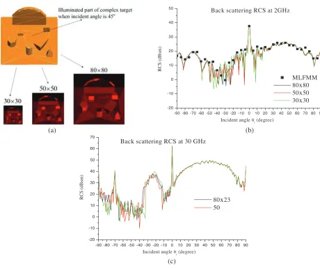
Figure 11(a) shows the illuminated part of the complex target when the incident angle is 45◦. And it also displays the images of pixel matrix with different sizes. When the pixel size is small, such as 30×30, the basic characteristics can be shown. With the pixel matrix getting larger, more details can be identified. Since the proposed method is feasible at high frequency, Figure 11(b) and Figure 11(c) show the HH polarization backscattering RCSs at 2 GHz and 30 GHz, respectively. The black line, red line and green line are results corresponding to the pixel matrix sizes of 80×80, 50×50, and 30×30, respectively. The differences of the three results are small. Table 3 gives the calculation time for different pixel matrices with i7-4790K CPU. When pixel matrix is 80×80, it takes 17.628 s to calculate results for 181 angles, which are from −90◦ to 90◦. When the size of pixel matrix becomes small, the calculation time decreases correspondingly. It only takes 9.063 s to calculate results when pixel matrix is 30×30. Thus, when the accuracy requirement is low, it is feasible to use a small size pixel matrix which is in the premise that the basic shape of model can be imaged.
Table 3. Total calculation time of 181 angles for different pixel matrices.
hhhhhhh
hhhhhhhhh
Patch number
Size of pixel matrix Calculation time (s) 30×30 50×50 80×80
216 9.063 9.182 17.628
The same model can be described with different sizes of patches. Figure 12(a) and Figure 12(b) present two models which have the same parameters but different patch sizes. Models 1 and 2 are subdivided into 216 and 3661 triangular patches, respectively. Figure 13(b) gives the RCS of the two models at 30 GHz. It is found that the calculated results of the two models have no significant difference. This is because the rectangular wave beam-based GO/PO method has no limitation for the model patch size. It only demands that the model is described accurately. However, more patches require more time to image the model. Table 4 lists the runtime for calculating results of 181 incident angles with i7-4790K CPU. The calculation time for model 1 is only 17.628 s which is about one tenth of model 2. Thus, decreasing the patch number is a better method of maximizing calculation efficiency based on the accuracy of the model.
-90 -80 -70 -60 -50 -40 -30 -20 -10 0 10 20 30 40 50 60 70 80 90 -20
-10 0 10 20 30 40 50
Back scattering RCS at 2GHz
RCS (dB
sm)
Incident angle θi (degree)
MLFMM 80x80 50x50 30x30
(a)
(b)
-90 -80 -70 -60 -50 -40 -30 -20 -10 0 10 20 30 40 50 60 70 80 90 -20
-10 0 10 20 30 40 50 60 70
Back scattering RCS at 30 GHz
80x23 50
(c)
Incident angle θi (degree)
RCS (dB
sm)
Figure 11. (a) Image of different sizes of pixel matrix, and HH-polarization RCS of complex target at 2.0 GHz, (c) 30 GHz.
; <
=
2m
2m
; <
=
2m
2m
(a) (b)
Figure 12. Model described by (a) large size patches, (b) small size patches.
in Figure 13(a), construct a right-angle corner, the reflection beams only play an important role at the angle near θi = −21◦. It is because Face 2 affects the reflection beams, and the influence is the least
when the incident angle θi equals −19.4◦.
; =
2m
0.75m Face 1
Face 2 Face 3
-80 -60 -40 -20 0 20 40 60 80 -20
0 20 40 60 80
i=-21 o
RC
S (dB
sm
)
Incident angle i (degree)
Model 1: Pure PO
Results with 2 reflections
Model 2: Pure PO
Results with 2 reflections
θ=−19.4ο
(a) (b)
θ
Figure 13. (a) Special incident angle, (b) RCS at 30 GHz.
Table 4. Calculation time with different number of patches.
hhhhhhhhhhhhhh
hh
Patch number
Size of pixel matrix Calculation time (s) 80×80
Model 1: 216 17.628
Model 2: 3661 167.973
-180 -150 -120 -90 -60 -30 0 30 60 90 120 150 180 -20
-10 0 10 20 30 40
RC
S
(
d
B
m
2)
Incident angle i (degree) Measured data
Calculated results
ϕ XY
Z
(a) (b)
Figure 14. (a) Model with curve surface, (b) RCS at 10 GHz.
calculation will increase too. Figure 14(a) shows the model composed of a sphere and a plate. The plate can be described by a large patch. However, the sphere must be described by small patch size. Figure 14(b) shows the RCS of the model at 10 GHz, along with the measured results [18]. When the pixel matrix is 100×100, the calculated RCS results fit well with the measured ones.
5. CONCLUSION
ACKNOWLEDGMENT
This work was supported in part by the Fundamental Research Funds for the Central Universities, the National Natural Science Foundation of China under Grant No. 61372004/41306188, the China Postdoctoral Science Foundation under Grant No. 2015M572524, and Shanghai Aerospace Science and Technology Innovation Fund (SAST2015008).
REFERENCES
1. Delgado, C., E. Garcia, J. Moreno, I. Gonzalez-Diego, and M. F. Catedra, “An overview of the evolution of method of moments techniques in modern EM simulators (invited paper),” Progress In Electromagnetics Research, Vol. 150, 109–121, 2015..
2. Guillod, T., F. Kehl, and C. V. Hafner, “FEM-based method for the simulation of dielectric waveguide grating biosensors,”Progress In Electromagnetics Research, Vol. 137, 565–583, 2013. 3. Balanis, C. A., Advanced Engineering Electromagnetics, Wiley, New York, 1989.
4. Knott, E. F., “RCS reduction of dihedral corners,”IEEE Trans. Antennas Propag., Vol. 25, No. 3, 406–409, 1977.
5. Yan, J., J. Hu, and Z. Nie, “Calculation of the physical optics scattering by trimmed NURBS surfaces,”IEEE Antennas Wireless Propag. Lett., Vol. 13, 1640–1643, 2014.
6. Kim, J. H., et al., “Analysis of FSS radomes based on physical optics method and ray tracing technique,”IEEE Antennas Wireless Propag. Lett., Vol. 13, 868–871, 2014.
7. Ufimtsev, P. Y., Fundamentals of the Physical Theory of Diffraction, Wiley, Hoboken, NJ, 2007. 8. Tsang, L., et al.,Scattering of Electromagnetic Waves (Vol. 2: Numerical Simulations), Viely, New
York, 2001.
9. Bucci, O. M., T. Isernia, and A. F. Morabito, “Optimal synthesis of circularly symmetric shaped beams,”IEEE Trans. Antennas Propag., Vol. 62, No. 4, 1954–1964, 2014.
10. Tao, Y. B., H. Lin, and H. J. Bao, “Kd-tree based fast ray tracing for RCS prediction,” Progress In Electromagnetics Research, Vol. 81, 329–341, 2008.
11. Tao, Y., H. Lin, and H. Bao, “GPU-based shooting and bouncing ray method for fast RCS prediction,”IEEE Trans. Antennas Propag., Vol. 58, No. 2, 494–502, 2010.
12. Ling, H., R. C. Chow, and S. W. Lee, “Shooting and bouncing rays: Calculating the RCS of an arbitrarily shaped cavity,” IEEE Trans. Antennas Propag., Vol. 37, No. 2, 194–205, 1989.
13. Wei, P. B., et al., “GPU-based combination of GO and PO for electromagnetic scattering from satellite,” IEEE Trans. Antennas Propag., Vol. 60, No. 11, 5278–5285, 2012.
14. Fan, T. Q. and L. X. Guo, “OpenGL-based hybrid GO/PO computation for RCS of electrically large complex objects,” IEEE Antennas Wireless Propag. Lett., Vol. 13, 666–669, 2014.
15. Sundararajan, P. and M. Y. Niamat, “FPGA implementation of the ray tracing algorithm used in the Xpatch software,”Proc. IEEE MWSCAS’01, Vol. 1, 446–449, Dayton, OH, Aug. 2001.
16. Jin, K.-S., T. Suh, S.-H. Suk, and H.-T. Kim, “Fast ray tracing using a space-division algorithm for RCS prediction,”Journal of Electromagnetic Waves and Applications, Vol. 20, No. 1, 119–126, Jan. 2006.
17. Rius, J. M., M. Ferrando, and L. Jofre, “GRECO: Graphical electromagnetic computing for RCS prediction in real time,”IEEE Antennas Propag. Mag., Vol. 35, No. 2, 7–17, 1993.