Progress In Electromagnetics Research M, Vol. 39, 151–159, 2014
Automatic Target Recognition Using Jet Engine Modulation
and Time-Frequency Transform
Sang-Hong Park*
Abstract—We propose a method to recognize targets by using the signature of jet engine modulation (JEM) generated by the rotating blades in jet engines. The method combines time-frequency transform, 2-dimensional (2D) principal component analysis, and a nearest-neighbor classifier. In simulations using five propellers composed of isotropic point scatterers, the proposed method was insensitive to signal-to-noise SNR variation; this insensitivity was a result of the effective 2D time-frequency feature and the noise suppression by the matched filter. In simulations using a reduced training database, the result was most sensitive to variation in the rotation velocity of the blades.
1. INTRODUCTION
Automatic target recognition (ATR) is a technique to detect and recognize a target by using data collected from a variety of radar sensors that use wide-band electromagnetic signals. ATR has been widely applied to classification of enemy jets in warfare. Mainly, two features have been used for ATR: high resolution range profile (HRRP) and inverse synthetic aperture radar image (ISAR). However, recent research results indicate that another signature called the micro-Doppler (m-D) phenomenon [1] has high potential for use in ATR [2].
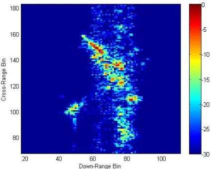
The basic principle for m-D is that rapid mechanical rotation and vibration components of a rigid body impose additional Doppler frequency modulation on the returned radar signal. The amount of frequency modulation isfD = 2v/λwherevis the relative velocity of the blade to the radar line of sight and λ the wavelength of the radar signal. For the ISAR image, this frequency modulation seriously blurs the image in cross-range direction (Figure 1), and therefore should be removed to enable ATR of the ISAR image. However, these noise-like components can also be exploited for ATR as a useful signature because they represent the time-varying frequency of the target.
m-D has been applied to target recognition. High-resolution time-frequency techniques can be used to extract the time-varying m-D signature [3]. The adaptive chirplet presentation can extract the m-D signature from an ISAR image of an aircraft [4] and image-processing algorithms such as the Radon transform [5] and the Hough transform (HT) [6] have been introduced to separate m-D features m-D analysis has been used to classify the type of helicopter blade [5] or automobile wheel [7], to analyze human gaits and wind farms [8, 9]. Recently, MD has been intensively applied to the recognition of the ballistic missile [10, 11].
The rotation of blades in a jet produces engine modulation (JEM) [2]. Each fighter jet is equipped with a unique engine that provides a distinct JEM signature that can used for ATR. In this paper, by using the mathematical modeling and the obtained characteristics of JEM, we identify a target based on time-frequency transform (TFT) and two-dimensional (2D) principle component analysis (PCA). A training database was constructed for each of the numerous regular increments of the aspect angle and the rotational velocity (RV). The test data were obtained at a random angle and a random RV. Then classification was conducted using a nearest neighbor classifier and a time-frequency signature
Received 7 October 2014, Accepted 2 November 2014, Scheduled 6 November 2014
* Corresponding author: Sang-Hong Park ([email protected]).
Figure 1. ISAR image of a Boeing747 contaminated by micro-Doppler frequency modulation.
compressed by 2D PCA. In simulations using five different propellers composed of isotropic point scatterers, the proposed method yielded high classification results even at low SNRs due to the effective 2D time-frequency feature.
2. MATHEMATICAL MODELING AND PROPOSED METHOD 2.1. Mathematical Modeling of JEM
Consider that a propeller composed of point scatters is placed on the y-axis and rotating around it at RVωR. The position of scatterer s on bladebin the propeller at slow-time tp is given by
x(t
p)bs y(tp)bs z(tp)bs
=
cos (ω
Rtp+φ0) 0 −sin (ωRtp+φ0)
0 1 0
sin (ωRtp+φ0) 0 cos (ωRtp+φ0)
x0bs
y0bs
z0bs
+ 0 ycen 0 , (1)
where [x0bs y0bs z0bs]T is the initial position of the scatterer, [0 ycen 0]T the position of the propeller center, andφ0the initial angle of the blade. Slow time is expressed in terms of the radar pulse repetition
interval (PRI) and is different from the fast timetfor the radar signal. If the scatter is seen at an aspect angle θto its local (x,y) coordinate, (1) becomes
x(t
p)θbs y(tp)θbs z(tp)θbs
=
cosθ −sinθ 0
sinθ cosθ 0
0 0 1
cos (ωRtp+φ0) 0 −sin (ωRtp+φ0)
0 1 0
sin (ωRtp+φ0) 0 cos (ωRtp+φ0)
x0bs
y0bs
z0bs
+ 0 ycen 0 , (2)
where [x(tp)θbs y(tp)θbs z(tp)θbs]T is the position of the scatterer at the an angleθ.
Assuming the plane wave approximation and the radar line of sight (RLOS) vector [0 1 0], the distance to son bat tp and θ is given by
r(tp)θbs=y(tp)θbs =x0bscos (ωRtp+φ0) sinθ−z0bssin (ωRtp+φ0) sinθ+ycen+y0bscosθ
+x0bssin (ωRtp+φ0) +z0bscos (ωRtp+φ0), (3)
which is a simple inner product of the RLOS vector and position vector. Then, the echo signalsR(t) of the transmitted radar signal with frequencyf becomes
sR(tp) = exp
j2πf
t−2r(tp)θbs c
= expj2πf0t+ Φ (tp)θbs , where Φ (tp)θbs=−
4πr(tp)θbs
λ . (4)
After baseband conversion, the frequency att caused by the rotating scatter becomes
f(tp)θbs=dΦ(tp)θbs dtp =−
4π
Progress In Electromagnetics Research M, Vol. 39, 2014 153
which is the sum of the sine and cosine functions ofωR. Thus, a time-frequency method is more efficient to describe the time-varying nature of JEM than is a simple FT method.
2.2. Rada Signal Modeling
For the radar signal, we assume a monostatic chirp waveform [12]
r(t) =A0ej
2πf0t+Bwt2τ2
×rect t τ , (6)
where r(t) is a transmitted signal at t,A0 its amplitude, f0 the start frequency, Bw the bandwidth,τ
the pulse duration, and rect = 1 ift−τ /2≤t≤t+τ /2 and 0 otherwise. At each pulse emission time tp, the received signal reflected from a propeller composed of B blades, each of which has S isotropic point scatterers, becomes
g(tp, t) = B b=1 S s=1
Absej2π
f0(t−r(tp)bs)+Bw(t−r2(τtp)bs)2
×rect
t−r(tp)bs τ
, (7)
where Abs is the amplitude of sin b, r(tp)bs the time delay between the radar and the scatterer at tp, andr(tp)bs is calculated using a plane wave approximation, in which the distance to a scattering center is that projected onto the RLOS vector. The discrete expression for (7) is
g[m, n] = B b=1 S s=1
Absej2π
f0(nTs−r(mT)bs)+B(nTs−r2(τmT)bs)2
×rect
nTs−r(mT)bs τ
, (8)
where Ts is the sampling period for the radar, T the pulse repetition interval (PRI), m is a fast-time index, andna slow-time index. The time-varying frequency of the JEM is sampled at the pulse repetition frequency (PRF) equal to 1/PRI, so high PRFs are required when sampling high JEM frequencies.
2.3. TFT and 2D PCA
TFT is used to represent the power distribution of the frequency of JEM over time. In this paper, we use the short-time Fourier transform (STFT) which is easily implemented by the simple fast FT. The input signal s(t) at timeτ is transformed by STFT to [13]:
STFT(t, f) =
∞
−∞s(τ)γ
∗(τ −t)e−j2πfτdτ , (9)
where f is the frequency and γ the window function. Because the sidelobe caused by the rectangular window may distort the MD image, we used the window function at the cost of increased resolution. In this paper, Hamming window was used. Other types of windows such as Hanning, Blackman, and spline windows can be used depending on the TFT method. In discrete form, (9) is expressed as
STFT[p, q] = L−1
k=0
s[k]γ [k−p]e−2πqkL , (10)
where k is the time index, L the window length, p sampled time index, andq the sampled frequency index.
Because the TFT image contains much redundant information, we apply 2D PCA to compress the image and to extract useful features that distinguish targets effectively. The main point of 2D PCA is to use a simple matrix multiplication
Y=AX, (11)
to project the TFT imageAonto the projection axesX, whereXis a set ofdeigenvectors of the image covariance matrix given by
Gt= 1 Mtr
Mtr
j=1
Aj−A¯T Aj−A¯, (12)
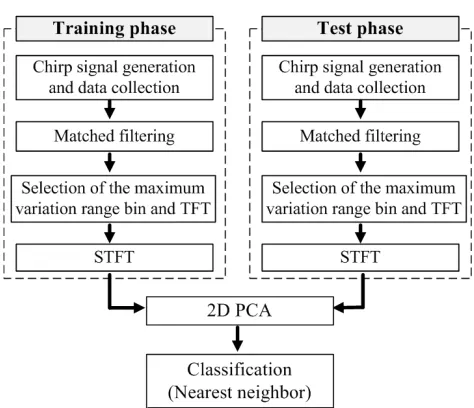
Figure 2. Proposed classification procedure. Figure 3. Test image clipping.
2.4. Proposed Recognition Method
The proposed method is composed a training phase and a test phase (Figure 2). In each phase, the collected radar signal in (8) is matched-filtered for each mto yield HRRP (Figure 2). To automatically select the range bin of JEM, we used the variation of the absolute value in the HRRP and selected the one that yielded the highest variation. Because the initial phases of the sinusoidal curve can differ between the training data and the test data, the test data require longer observation time to find the maximum match than do the training data.
In the second step, STFT is conducted using the signal in the selected range bin to construct the training and test TFT images. Due to the longer observation time for the data, the test TFT image has a longer time axis than the training TFT image when the frequency axes are equal. In classification, the training and test images are compressed by 2D PCA, and the test image is classified by a simple nearest neighbor whose classification rule is as follows:
ˆi= min
i Yu−Yi, (13)
whereYu is the compressed 2D PCA image of an unknown target, andYi is that of the training image of the ith target, and · is the Frobenius norm [15]. The Frobenius norm of a ma×na matrixA is given by
A=
ma
i=1
na
j=1
|aij|2. (14)
Because of the size difference between the training and test images, the test TFT image is clipped using a window with the training image size, shifting from the 1st column of the test image to the last (Figure 3). For each shifta, the clipped image is divided byA(14) to remove the amplitude variation, then 2D PCA is applied to deriveYua and Yua−Yi. Finally, the minimum value ofYua−Yiis used asYu−Yi for theith target.
3. SIMULATION RESULT
Progress In Electromagnetics Research M, Vol. 39, 2014 155
(a) (b)
(c) (d)
(e)
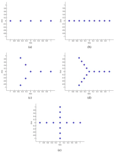
Figure 4. Propeller targets used for simulation. (a) Target 1. (b) Target 2. (c) Target 3. (d) Target 4. (e) Target 5.
to achieve the desired signal-to-noise ratio (SNR).dfor 2D PCA in (11) was set to 2 because this value gives good classification results [17]. Classification accuracy was expressed as the correct classification percentage
Pc =Mc/Mtr×100%, (15)
whereMc is the number of correct classifications, and Mtr is the same as in (12).
In constructing TFT images from the sampled JEM data in a range bin with the maximum signal variation, the 50-point Hamming window was used with an overlap of 40 points between each pair of neighboring time samples. Each 50-point set of windowed data was zero-padded to 2048 points, and fast FT was conducted to construct the TFI for each time shift.
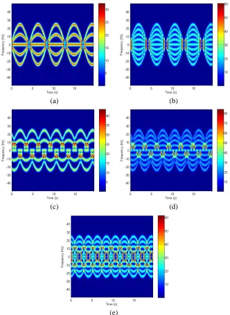
The TFT images of targets at θ = 30◦ and rotating at RPM = 7 consisted of sinusoidal waves
(c)
(a) (b)
(d)
(e)
Progress In Electromagnetics Research M, Vol. 39, 2014 157
caused by the rotation of each scatterer (Figure 5). Each wave had an amplitude that corresponded to the distance of the scatterer from the center, and phases of the waves were offset by an amount that corresponded to the angle between pairs of blades; i.e., a constant line (amplitude 0) for the central scatterer, and two or four additional waves offset by 180◦ (Target 1, Figure 5(a); Target 2, Figure 5(b)), 120◦ (Target 3, Figure 5(c); Target 4, Figure 5(d)), or 90◦ (Target 5, Figure 5(e)).
The simulation result for various SNRs (0∼30 dB with 10 dB increment) with Δθ = 1◦ and ΔRP M = 1 was very stable and degraded as SNR decreased (Figure 6). However, the degree of degradation was very small (Pc remained > 95%) because of noise suppression by the matched-filter. The effective 2D features of the TFI image also contributed to the high Pc at low SNR. This result proves that JEM can be very effective for ATR.
In simulations using 1≤Δθ≤10 in increments of 1 with SNR = 30 dB and ΔRPM = 1, the result was more sensitive to variation of Δθthan to variation of SNR (Figure 7). Due to the reduced size of the training database, Pc decreased as Δθincreased. Pc was 89.2% for Δθ≥5◦, so Δθ should be<5◦ to achieve Pc >90%.
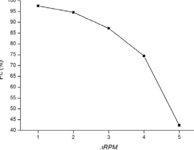
Pc was most sensitive to ΔRPM variation as it was varied from 1 to 5 with an increment 1 with Δθ = 1◦ and SNR = 30 dB. The sharp degradation in Pc (Figure 8) was due to the scaling of the sinusoidal curves in the TFT image. Because the sinusoidal curves in the TFT image can be scaled or expanded depending on the RPM, the result was most affected by RPM. The simulations suggest that ΔRPM should be<3 (50% of the total RPM range) to achievePc>90%. However this value of ΔRPM is not absolute because at very high RPMs, this small ΔRPM would not considerably affect the
Figure 6. Percent correct identification vs. SNRs.
Figure 7. Percent correct identification vs. Δθ.
shape of a TFI image; further investigations using several RPM ranges should be conducted to define this range more definitively.
4. CONCLUSION
We proposed an efficient method composed of range compression, TFT, 2D PCA and the nearest neighbor classifier to recognize targets using their JEM signatures. The time-varying frequency of JEM signal due to the rotation of the propeller was proved by the signal model, and high classification accuracy was obtained in simulations using five propeller models that consisted of isotropic scatterers. The simulation result was insensitive to SNR variation and was sensitive to Δθ and ΔRPM; the result was more dependent on ΔRPM than on Δθdue to the variation of sinusoidal curves in the TFT image. For ΔRPM, further investigations are required using several RPM ranges.
This paper provides strong evidence that the JEM signature can be applied to ATR to identify jets. However, it should not be used alone, but used with other features such as 2D ISAR image. When the aircraft closes directly toward the radar, ISAR image cannot provide useful features for ATR because of the high elevation angle [18]. In this case, the JEM signal collected from the observed propeller will significantly improve the classification result. Our next research will focus on fusion of the two features when a jet moves directly toward the radar.
ACKNOWLEDGMENT
This research was supported by Basic Science Research Program through the National Research Foundation of Korea (NRF) funded by the Ministry of Education, Science and Technology (2012R1A1A1002047).
REFERENCES
1. Chen, V. C., F. Li, S. S. Ho, and H. Wechsler, “Micro-Doppler effect in radar: Phenomenon, model, and simulation study,”IEEE Trans. Aerosp. Electron. Syst., Vol. 42, No. 1, 2–21, Jan. 2006. 2. Tait, P., Introduction to Radar Target Recognition, IET, 2005.
3. Thayaparan, T., S. Abrol, E. Riseborough, L. Stankovic, D. Lamothe, and G. Duff, “Analysis of radar micro-Doppler signatures from experimental helicopter and human data,” IET Radar Sonar Navig., Vol. 1, No. 4, 289–299, Aug. 2007.
4. Li, J. and H. Ling, “Application of adaptive chirplet representation for ISAR feature extraction from targets with rotating parts,” Proc. Inst. Elect. Eng. Radar Sonar Navig., Vol. 150, No. 4, 284–291, Aug. 2003.
5. Stankovic, L., I. Djurovic, and T. Thayaparan, “Separation of target rigid body and micro-Doppler effects in ISAR imaging,”IEEE Trans. Aerosp. Electron. Syst., Vol. 42, No. 4, 1496–1506, Oct. 2006. 6. Zhang, Q., T. S. Yeo, H. S. Tan, and Y. Luo, “Imaging of a moving target with rotating parts based on the Hough transform,”IEEE Trans. Geosci. Remote Sens., Vol. 46, No. 1, 291–299, Jan. 2008. 7. Ghaleb, A., L. Vignaud, and J. M. Nicolas, “Micro-Doppler analysis of wheels and pedestrians in
ISAR imaging,”IET Signal Process., Vol. 2, No. 3, 301–311, Sep. 2008.
8. Kim, Y. and H. Ling, “Human activity classification based on micro-Doppler signatures using a support vector machine,”IEEE Trans. Geosci. Remote Sens., Vol. 47, No. 5, 1328–1337, May 2009. 9. Jung, J. H., U. Lee, S. H. Kim, and S. H. Park, “Micro-Doppler analysis of Korean offshore wind
turbine on the L-band radar,”Progress In Electromagnetics Research, Vol. 143, 87–104, 2010. 10. Jung, J. H., K. T. Kim, S. H. Kim, and S. H. Park, “Micro-Doppler extraction and analysis of
the ballistic missile using RDA based on the real flight scenario,” Progress In Electromagnetics Research M, Vol. 37, 83–93, 2014.
Progress In Electromagnetics Research M, Vol. 39, 2014 159
13. Qian, S.,Time-freqency and Wavelet Transforms, Prentice Hall PTR, 2002.
14. Yang, J., D. Zhang, A. F. Frangi, and J.-Y. Yang, “Two-dimensional PCA: A new approach to appearance-based face representation and recognition,”IEEE Trans. Pattern Analysis and Machine Intelligence, Vol. 26, 131–137, Jan. 2004.
15. Golub, G. H. and C. F. Van Loan, Matrix Computations, The Johns Hopkins University Press, 1996.
16. Zyweck, A., “Preprocessing issues in high resolution radar target classification,” Ph.D. Thesis, University of Adelaide, Australia, 1995.
17. Han, S.-K., H.-T. Kim, S.-H. Park, and K.-T. Kim, “Efficient radar target recognition using a combination of range profile and time-frequency analysis,” Progress In Electromagnetics Research, Vol. 108, 131–140, 2010.