Identification of groundwater discharge along the shoreline of large inland lakes in Southern Ontario

Scholarship@Western

Scholarship@Western

Electronic Thesis and Dissertation Repository

6-2-2016 12:00 AM

Identification of groundwater discharge along the shoreline of

Identification of groundwater discharge along the shoreline of

large inland lakes in Southern Ontario

large inland lakes in Southern Ontario

Tao Ji

The University of Western Ontario Supervisor

Clare Robinson

The University of Western Ontario

Graduate Program in Civil and Environmental Engineering

A thesis submitted in partial fulfillment of the requirements for the degree in Master of Engineering Science

© Tao Ji 2016

Follow this and additional works at: https://ir.lib.uwo.ca/etd

Part of the Environmental Engineering Commons

Recommended Citation Recommended Citation

Ji, Tao, "Identification of groundwater discharge along the shoreline of large inland lakes in Southern Ontario" (2016). Electronic Thesis and Dissertation Repository. 3773.

https://ir.lib.uwo.ca/etd/3773

This Dissertation/Thesis is brought to you for free and open access by Scholarship@Western. It has been accepted for inclusion in Electronic Thesis and Dissertation Repository by an authorized administrator of

Abstract

identify groundwater discharge hotspots along 80 km of shoreline. Two potential groundwater discharge hotspot areas were identified, as well as two areas where indirect groundwater discharge (i.e. groundwater discharge to creeks which then flows into the lake) may affect the nearshore lake water quality. High spatial resolution surveys were conducted in the groundwater discharge hotspot areas with data indicating that groundwater discharge in these areas is higher near the shoreline and decreases offshore. Groundwater discharge rates in Lake Simcoe were estimated to range from 0.18 ± 0.01 - 4.18 ± 0.30 m3 _m-1 _d-1 _{from applying the} steady-state 222_{Rn mass balance model. The} 222_{Rn concentrations in the lake exhibited high} temporal variability with preliminary analysis indicating this variability is due to varying wind speed and, to a lesser extent, precipitation. Better understanding of factors contributing to the temporal variability in 222_{Rn concentrations is needed for more accurate interpretation of the} regional-scale 222_{Rn survey data. The combination of field methods evaluated in this thesis} provides characterization of nearshore groundwater discharge to large inland lakes at multiple scales as required to develop more effective management plans to mitigate the contribution of groundwater pollutant inputs to nearshore waters.

Keywords

iii

Co-Authorship Statement

The candidate is responsible for the collection and analysis of field data as well as writing all thesis chapters. Dr. Clare Robinson provided the initial motivation for this research, assisted with field work, and provided suggestions for data analysis and improvement of the thesis. The co-authorship breakdown of Chapters 3 and 4 are as follows:

Chapter 3: Multiple methods for characterizing groundwater discharge along a Lake Huron shoreline

Authors: Tao Ji, Richard Peterson, Kevin Befus, Clare Robinson Contributions:

Tao Ji: Designed the field deployment plan, built and set up all field equipment except for the 222_{Rn detection system and ERT survey equipment, and measured, analyzed and interpreted} field data, performed lab experiment, and wrote the thesis chapter.

Richard Peterson: Together with Tao Ji, was responsible for conducting the 222_{Rn survey, and} provided advice for analysis of 222_{Rn survey data.}

Kevin Befus: Conducted the regional-scale ERT survey and ER inversion modeling.

Clare Robinson: Initiated research topic, aided in field investigations, provided advice for data analysis and revised the chapter draft.

Chapter 4: Using 222_{Rn as a tracer to quantify groundwater discharge along the Lake Simcoe} shoreline

Authors: Tao Ji, Clare Robinson

Tao Ji: Designed the field deployment plan, built field equipment and instrumentation, measured, analyzed and interpreted field data, performed laboratory experiment and wrote the thesis chapter.

Acknowledgments

This thesis would not have been completed without the help of many people.

Firstly, I would like to express my sincere gratitude to my supervisor Dr. Clare Robinson who offered me this exciting research opportunity. I admire her intelligence and meticulous working attitude. She is always patient and willing to provide positive feedback. Her guidance, motivation and immense knowledge has been involved in each step of my progress.

I also would like to thank all members of the RESTORE research group. It is my honor to be a part of it and study in such an encouraging and friendly environment. I have obtained so many supports from RESTORE since I arrived in Canada. I want to acknowledge Drs. Jason Gerhard and Denis O’Carroll who provided me with numerous useful scientific advices and guidance for my improvement.

Thanks to Dr. Richard Peterson and his Ph.D student Leigha Peterson, as well as Dr. Kevin Befus who gave me much guidance and assistance for field work and data analysis in my research. Thanks to Tim Krsul, Matt McNeice and other staff from MOECC in Barrie who made my research move smoothly and successfully.

A special thanks to my great field work partners - Spencer Malott, Taryn Fournie, Hayley Wallace, Brandon Powers, Victoria Trglavcnik, Alex Han, Borna Mahmoudian and Laura Vogel. I will forever remember those happy days we spent together at the beaches and on the boat.

Thanks for the supports and helps from all of the faculty and staff in the Department of Civil and Environmental Engineering.

Thanks to all of the teammates from my volleyball team in London for sharing the happiness and athletic experiences.

v

Table of Contents

Abstract ... i

Co-Authorship Statement... iii

Acknowledgments... iv

Table of Contents ... v

List of Table ... viii

List of Figures ... ix

Chapter 1 ... 1

1 Introduction ... 1

1.1 Research background ... 1

1.2 Research objective ... 3

1.3 Thesis outline ... 3

1.4 References ... 5

Chapter 2 ... 8

2 Literature review ... 8

2.1 The importance of groundwater discharge to large inland lakes ... 8

2.1.1 Groundwater discharge to the Laurentian Great Lakes ... 10

2.1.2 Groundwater discharge to Lake Simcoe ... 12

2.2 Methods to quantify groundwater discharge to large inland lakes ... 14

2.2.1 222_{Rn as a tracer ... 15}

2.2.2 Groundwater hydraulic gradient ... 19

2.2.3 Heat as a tracer ... 21

2.2.4 Electrical Resistivity Tomography (ERT) ... 24

2.3 References ... 26

3 Multiple methods for characterizing groundwater discharge along a Lake Huron

shoreline ... 39

3.1 Introduction ... 39

3.2 Study site description ... 41

3.3 Methods... 43

3.3.1 Regional-scale measurements ... 43

3.3.2 Local-scale measurements ... 49

3.4 Results and discussion ... 52

3.4.1 Regional-scale 222_{Rn and ERT survey ... 52}

3.4.2 High resolution 222_{Rn survey ... 55}

3.4.3 Local-scale groundwater discharge measurements ... 59

3.4.4 Comparison of methods ... 62

3.5 Conclusions ... 65

3.6 References ... 66

Chapter 4 ... 72

4 Using 222_{Rn as a tracer to quantify groundwater discharge along the shoreline of Lake} Simcoe ... 72

4.1 Introduction ... 72

4.2 Study site description ... 75

4.3 Methods... 79

4.3.1 222_{Rn boat surveys ... 79}

4.3.2 222_{Rn mass balance calculations... 80}

4.3.3 Hydraulic gradient measurements... 84

4.4 Results and discussion ... 85

4.4.1 Regional-scale 222_{Rn survey results ... 85}

4.4.2 High-resolution 222_{Rn survey results ... 97}

vii

4.4.4 Factors affecting temporal variability of in-lake 222_{Rn concentrations .. 102}

4.5 Conclusions ... 105

4.6 Reference ... 107

Chapter 5 ... 112

5 Summary and recommendations ... 112

5.1 Summary ... 112

5.2 Recommendations ... 114

Appendices ... 116

Appendix 1: Estimation of hydraulic conductivity ... 116

Appendix 2: 222_{Rn survey results in Nottawasaga Bay ... 118}

Appendix 3: Sensitivity analysis for 222_{Rn atmosphere evasion ... 120}

Appendix 4: Upland till landforms and tunnel channel aquifers ... 121

Appendix 5: 222_{Rn concentrations in groundwater endmembers along Lake Simcoe .... 122}

Appendix 6: 222_{Rn survey results in Lake Simcoe ... 123}

List of Table

Table 2-1: Summary of studies of direct groundwater discharge to the Great Lakes. ... 12 Table 3-1: Estimated groundwater discharge (Qgd, m3 m-1 d-1) determined by four

measurement techniques at six locations along the shoreline of Nottawasaga Bay. “/” means no data is available. ... 64 Table 4-1: Total groundwater discharge from subwatersheds to Lake Simcoe estimated using numerical groundwater models developed for ESGRA assessments. Groundwater discharge per m of shoreline (Qgd) is calculated based on the estimated shoreline length for each

subwatershed. ... 74 Table 4-2: 222_{Rn concentration and base flow index (BFI) measured in creeks discharging in} Lake Simcoe in the study area. The error shown for the 222_{Rn concentrations is the 2σ}

uncertainty. “/” means no data is available. ... 86 Table 4-3: Input parameter values and results for estimation of Qgd based on groundwater

ix

List of Figures

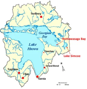
Figure 2-1: Generalized direct and indirect groundwater flow systems in the Great Lakes Region (figure modified from Grannemann et al., 2000). ... 9 Figure 2-2: Map showing location of Nottawasaga Bay in Lake Huron and Lake Simcoe (figure modified from Northeast Michigan Lake Huron Watershed, 2014). ... 9 Figure 2-3: 222_{Rn mass balance model for estimating groundwater discharge (modified from} Burnett and Dulaiova, 2003). The sources of 222_{Rn to the water column include groundwater} discharge (Jgw); diffusive flux of 222Rn from sediments (Jdiff) and222Rn production from 226Ra

(Jprod). The losses include mixing with offshore waters (Jmix); atmospheric evasion (Jatm) and

in-situ decay of 222_{Rn (Jdecay). ... 16} Figure 2-4: Schematic of “temperature stick”: six thermocouples attached to a metal stake and a datalogger to measure vertical temperature profiles below the sediment-water interface. One extra thermocouple was used to measure the surface water temperature. ... 22

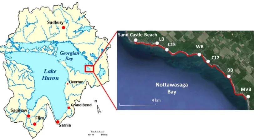
Figure 3-1: Map of the Lake Huron and Georgian Bay showing the location of the study area in Nottawasaga Bay near the Township of Tiny (red box) and track of regional-scale offshore 222_{Rn and ERT survey (red line). Map on left is reproduced from Northeast Michigan Lake} Huron Watershed (2014). The six locations where local-scale groundwater discharge

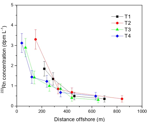
Figure 3-5: 222_{Rn concentrations measured in the high-resolution survey. The white dots} represent the beach sites where local-scale groundwater discharge measurements were conducted. 222_{Rn concentrations vs. distance offshore are shown in Figure 3-6 for the four} shore-normal transects indicated (black lines, T1-T4). ... 56 Figure 3-6: 222_{Rn concentrations from the high-resolution} 222_{Rn survey as a function of} distance offshore. The error bars show the 2σ uncertainty for the measured 222_Rn

concentrations. Locations of the four shore-normal transects, T1-T4, are shown in Figure 3-5. ... 57 Figure 3-7: qgd calculated from high-resolution 222Rn survey data. The colored dots represent

the sampling points with the color indicating the calculated qgd value. The numbers adjacent

to the dots represent the sampling point number with data provided in Table A2-1. The white dots show the beach sites where local-scale groundwater discharge measurements were conducted. The white lines are the transects where Qgd were calculated for C15 and LB. .... 58

Figure 3-8: Groundwater level (blue line) and sand surface profiles (black line) at the six study sites. The filled blue squares represent the locations of the wells. The horizontal hydraulic gradient ( ℎ ) was calculated from the groundwater level measurements at each site. ... 60 Figure 3-9: Specific flux (qgd) as a function of distance offshore for Balm Beach (BB) and

Mountain View Beach (MVB). Data was obtained at field sites in June 25th_{, 2014 using} vertical nested mini-piezometers. ... 61 Figure 3-10: (a) Vertical temperature profiles measured at BB in June 25th_{, 2014 and (b)} specific flux (qgd) estimated from vertical temperature profiles as a function of distance

xi

Figure 4-2: Map of subwatershed areas and stream network of Lake Simcoe. The red dots represent the creeks that were sampled for 222_{Rn concentrations. Figure modified from The} Louis Berger Group Inc. (2010)... 78 Figure 4-3: In-lake 222_{Rn concentrations from regional-scale survey conducted along the} shore of Kempenfelt Bay on (a) June 9th _{(yellow numbers) and 11}th _{(white numbers) 2015,} and (b) July 6th _{(white) and 8}th _{(yellow), 2015. The filled circles represent the measurement} locations and their colour indicate the 222_{Rn concentration range. The red box labeled (A) in} (a) indicates the area where a high-resolution survey was completed on July 10th_{, 2015. ... 88} Figure 4-4: In-lake 222_{Rn concentrations from regional-scale survey conducted along the} shore of Innisfil Area on (a) July 8th _{and (b) August 12}th_{, 2015. The filled circles represent} the measurement locations with their colour indicating the 222_{Rn concentration range. ... 89} Figure 4-5: In-lake 222_{Rn concentrations from regional-scale survey conducted along the} shore of Georgina Area on (a) August 13th_{, 2015 and (b) September 23}rd_{, 2015. The filled} circles represent the measurement locations with their colour indicating the 222_Rn

concentration range. The red box (B) and (C) in (a) indicates the area where high-resolution surveys were completed on September 24th _{and 25}th_{, 2015, respectively... 90} Figure 4-6: Groundwater endmember sampling locations (yellow dots) with the range of measured 222_{Rn concentrations (dpm L}-1_{) shown in brackets. All data is provided in Table} A5-1, Appendix 5... 92 Figure 4-7: In-lake Qgd from regional-scale survey conducted along the shore of Kempenfelt

Bay on (a) June 9th _{(yellow) and 11}th _{(white) 2015, and (b) July 6}th _{(white) and 8}th _(yellow), 2015. The filled circles represent the measurement locations and their colour indicate the Qgd

range. All data is provided in Table A6-1, Appendix 6. ... 94 Figure 4-8: In-lake Qgd from regional-scale survey conducted along the shore of Innisfil Area

on (a) July 8th _{and (b) August 12}th_{, 2015. The filled circles represent the measurement} locations with their colour indicates the Qgd range. All data is provided in Table A6-2,

Figure 4-9: In-lake Qgd from regional-scale survey conducted along the shore of Georgina

Area on (a) August 13th_{, 2015 and (b) September 23}rd_{, 2015. The filled circles represent the} measurement locations with their colour indicating the Qgd. All data is provided in Table

A6-3, Appendix 6. ... 96 Figure 4-10: In-lake 222_{Rn concentrations measured in high-resolution surveys conducted in} (a) Area A on July 10th_{, (b) Area B on September 24}th _{and (c) Area C on September 25}th_{. The} filled circles represent the measurement locations with their colour indicating the 222_Rn concentration range. All data is provided in Table A6-4, Appendix 6. ... 98 Figure 4-11: In-lake qgd measured in high-resolution surveys conducted in (a) Area A on July

10th _{and (b) Area C on September 25}th_{. The filled circles represent the measurement locations} with their colour indicating the qgd range. ... 100

Chapter 1

1

Introduction

1.1 Research background

Groundwater accounts for over 30% of the world’s freshwater (Shlklomanov, 1993). Almost nine million Canadians (30.3 % of the population) and 45.8 % of the population in Ontario rely on groundwater for municipal, domestic and rural use (Environment Canada, 2016). Despite its abundance and significance, groundwater is increasingly threatened by contamination caused by anthropogenic activities (Kalbus et al., 2006, Kidmose et al., 2015). Groundwater and surface water are inextricably linked and any changes in groundwater resources (water quantity or quality) can lead to the deterioration of surface waters and the related ecosystems (Grannemann et al., 2000). In response to the degraded water quality in many large inland lakes including the Laurentine Great Lakes (herein called the Great Lakes), there is an increasing need to evaluate the contribution of groundwater discharge in delivering contaminants into the lake. This information is required for the development of more effective water quality management programs.

Kornelsen and Coulibaly, 2014). LGD has been shown to play an important role in geochemical cycling and ecosystem functioning in lakes (Hayashi and Rosenberry, 2002, Meinikmann et al., 2013). For instance, many studies have shown that discharge of nutrient-enriched groundwater can alter the nutrient budget of lakes, leading to serious lake eutrophication issues (Grannemann et al., 2000, Kornelsen and Coulibaly, 2014, Meinikmann et al., 2015). Nutrients-driven lake eutrophication problems such as harmful and nuisance algae blooms have raised considerable public awareness and concern recently (Shaw et al., 1990, Evans et al., 1996, Winter et al., 2007, North et al., 2013, Kidmose et al., 2015). Although the importance of groundwater discharge to lakes is now widely recognized, groundwater inputs are still poorly understood and quantified for most lakes especially for large inland lakes such as the Great Lakes and Lake Simcoe. Identifying and quantifying groundwater discharge and associated pollutant loading is complex and challenging due to the difficulties in measuring these unseen fluxes (Burnett et al., 2006).

multiple methods be used in evaluating groundwater discharge (Burnett et al., 2006, Kalbus et al., 2006).

1.2 Research objective

This thesis is divided into three objectives. The first objective is to evaluate suitable field techniques for quantifying groundwater discharge into large inland lakes at different spatial scales (regional and local). The second objective is to evaluate the spatial patterns and quantities of groundwater discharge along shorelines of large inland lakes in Southern Ontario and link observed discharge groundwater patterns to hydrogeological characteristics of the nearshore area. The main field technique evaluated in this thesis for assessment of regional-scale groundwater discharge is the natural tracer 222_{Rn. The third objective, related to reducing} uncertainty in this measurement techniques, is to evaluate the causes of temporal variability of 222_{Rn concentrations in the lake water. Understanding large scale groundwater discharge}

patterns is the first critical step to better characterizing and quantifying groundwater as a potentially important non-point pollution source. The research presented in this thesis provides valuable information for water resource management in the study areas as well as methodologies that may be broadly applied to investigate groundwater discharge into large inland lakes.

1.3 Thesis outline

A concise description of the outline of this thesis is as follows:

Chapter 1: Introduction of the research background and research objectives.

Chapter 2: Literature review of previous work conducted to evaluate groundwater discharge into large inland lakes with a focus on applicable groundwater discharge measurement techniques and tools.

shorelines areas with high groundwater discharge and shows how a combination of approaches can be used to estimate groundwater discharge rates and evaluate spatial variability in groundwater discharge.

Chapter 4: Application of multiple field methods to quantify nearshore groundwater discharge into Lake Simcoe. Field results are used to identify groundwater discharge hotspots and to evaluate factors controlling the temporal variability of 222_{Rn concentrations in the lake water.}

1.4 References

ANDERSON, M. P. 2005. Heat as a ground water tracer. Ground Water, 43, 951-68.

BURNETT, W. C., AGGARWAL, P. K., AURELI, A., BOKUNIEWICZ, H., CABLE, J. E., CHARETTE, M. A., KONTAR, E., KRUPA, S., KULKARNI, K. M., LOVELESS, A., MOORE, W. S., OBERDORFER, J. A., OLIVEIRA, J., OZYURT, N., POVINEC, P., PRIVITERA, A. M., RAJAR, R., RAMESSUR, R. T., SCHOLTEN, J., STIEGLITZ, T., TANIGUCHI, M. & TURNER, J. V. 2006. Quantifying submarine groundwater discharge in the coastal zone via multiple methods. Science of the Total Environment,

367, 498-543.

BURNETT, W. C., PETERSON, R., MOORE, W. S. & DE OLIVEIRA, J. 2008. Radon and radium isotopes as tracers of submarine groundwater discharge – Results from the

Ubatuba, Brazil SGD assessment intercomparison. Estuarine, Coastal and Shelf

Science, 76, 501-511.

DIMOVA, N. T., BURNETT, W. C., CHANTON, J. P. & CORBETT, J. E. 2013. Application of radon-222 to investigate groundwater discharge into small shallow lakes. Journal of Hydrology, 486, 112-122.

ENVIRONMENT CANADA. 2016. Groundwater [Online]. Available:

https://www.ec.gc.ca/eau-water/default.asp?lang=En&n=300688DC-1.

EVANS, D. O., NICHOLLS, K. H., ALLEN, Y. C. & MCMURTRY, M. J. 1996. Historical land use, phosphorus loading, and loss of fish habitat in Lake Simcoe, Canada.

Canadian Journal of Fisheries and Aquatic Sciences, 53, 194-218.

GRANNEMANN, N. G., HUNT, R. J., NICHOLAS, J. R., REILLY, T. E. & WINTER, T. C.

2000. The Importance of Ground Water in the Great Lakes Region. Water-Resources

Investigations Report 2000-4008. Lansing, Michigan: U.S. Geological Survey.

HAYASHI, M. & ROSENBERRY, D. O. 2002. Effects of ground water exchange on the hydrology and ecology of surface water. Ground Water, 40, 309-16.

KALBUS, E., REINSTORF, F. & SCHIRMER, M. 2006. Measuring methods for groundwater? surface water interactions: a review. Hydrology and Earth System Sciences Discussions, 10, 873-887.

KIDMOSE, J., ENGESGAARD, P., OMMEN, D. A., NILSSON, B., FLINDT, M. R. & ANDERSEN, F. O. 2015. The Role of Groundwater for Lake-Water Quality and Quantification of N Seepage. Ground Water, 53, 709-21.

LEWANDOWSKI, J., MEINIKMANN, K., RUHTZ, T., PÖSCHKE, F. & KIRILLIN, G. 2013. Localization of lacustrine groundwater discharge (LGD) by airborne measurement of thermal infrared radiation. Remote Sensing of Environment, 138, 119-125.

MEINIKMANN, K., LEWANDOWSKI, J. & HUPFER, M. 2015. Phosphorus in groundwater discharge–A potential source for lake eutrophication. Journal of Hydrology, 524, 214-226.

MEINIKMANN, K., LEWANDOWSKI, J. & NÜTZMANN, G. 2013. Lacustrine groundwater discharge: Combined determination of volumes and spatial patterns. Journal of Hydrology, 502, 202-211.

MOORE, W. S. 1996. Large groundwater inputs to coastal waters revealed by 226Ra enrichments. Nature, 380, 612-614.

NORTH, R. L., BARTON, D., CROWE, A. S., DILLON, P. J., DOLSON, R. M. L., EVANS, D. O., GINN, B. K., HAKANSON, L., HAWRYSHYN, J., JARJANAZI, H., KING, J. W., LA ROSE, J. K. L., LEON, L., LEWIS, C. F. M., LIDDLE, G. E., LIN, Z. H., LONGSTAFFE, F. J., MACDONALD, R. A., MOLOT, L., OZERSKY, T., PALMER, M. E., QUINLAN, R., RENNIE, M. D., ROBILLARD, M. M., RODE, D., RUHLAND, K. M., SCHWALB, A., SMOL, J. P., STAINSBY, E., TRUMPICKAS, J. J., WINTER, J. G. & YOUNG, J. D. 2013. The state of Lake Simcoe (Ontario, Canada): the effects of multiple stressors on phosphorus and oxygen dynamics. Inland Waters, 3, 51-74. ONO, M., TOKUNAGA, T., SHIMADA, J. & ICHIYANAGI, K. 2013. Application of

continuous 222Rn monitor with dual loop system in a small lake. Ground Water, 51,

706-13.

POVINEC, P. P., BOKUNIEWICZ, H., BURNETT, W. C., CABLE, J., CHARETTE, M., COMANDUCCI, J.-F., KONTAR, E., MOORE, W. S., OBERDORFER, J. & DE OLIVEIRA, J. 2008. Isotope tracing of submarine groundwater discharge offshore

Ubatuba, Brazil: results of the IAEA–UNESCO SGD project. Journal of

Environmental Radioactivity, 99, 1596-1610.

SHAW, R., SHAW, J., FRICKER, H. & PREPAS, E. 1990. An integrated approach to quantify

groundwater transport of phosphorus to Narrow Lake, Alberta. Limnology and

Oceanography, 35, 870-886.

SHLKLOMANOV, I. A. 1993. Water in crisis: a guide to the world's fresh water resources.

In: GLEICK, P. H. (ed.). New York: Oxford University Press, Inc.

Chapter 2

2

Literature review

2.1 The importance of groundwater discharge to large inland

lakes

Figure 2-1: Generalized direct and indirect groundwater flow systems in the Great Lakes Region (figure modified from Grannemann et al., 2000).

2.1.1 Groundwater discharge to the Laurentian Great Lakes

The Great Lakes which include Lake Huron, Lake Ontario, Lake Superior, Lake Michigan and Lake Erie, holds 18-20% of the world’s freshwater supplies. Aquifers in the Great Lakes Basin also contain large volumes of groundwater - approximately 4,200 km3 _{- which is a major} resource and an important link between the Great Lakes and their watersheds (Grannemann et al., 2000). Nearshore waters of the Great Lakes are of immense ecological, economical and recreational value (Austin et al., 2007). These areas, however, are being increasingly threatened by deteriorated water quality (Cherkauer and McKereghan, 1991, Haack et al., 2005). For instance, increasingly large harmful cyanobacterial blooms have been observed annually since 1995 in the western basin of Lake Erie (Bails et al., 2006, Rinta-Kanto et al., 2005). In 2014, these blooms caused the shutdown of the drinking water distribution system in the City of Toledo for successive days impacting over half a million people (Rinta-Kanto et al., 2005, Berman, 2014, Obenour et al., 2014, Steffen et al., 2014). While water quality management efforts have historically focused on mitigating point pollution sources, there is increasing recognition that non-point sources including groundwater discharge may play an important role in delivering pollutants to nearshore waters (Hartmann, 1990, Mitsch and Wang, 2000, International Joint Commission, 2012). Despite this increasing recognition, the magnitude of direct groundwater discharge and associated pollutant loading to nearshore areas of the Great Lakes remains poorly understood.

et al., 2000, Haack et al., 2005). Studies have reported that non-point source chloride (Cl-_{) and} nitrate (NO3-) flow through the shallow aquifers into the Great Lakes (Hill, 1990, Boutt et al., 2001). For instance, Cherkauer et al. (1992) applied a two-dimensional finite-element transport

model in Door Peninsula, Wisconsin and estimated that around 33% and 38% of the total Cl

-and NO3- that entered the surficial aquifer of the Green Bay Basin was transported into Lake Michigan via direct groundwater discharge.

Prior studies have attempted to quantify direct groundwater discharge to the Great Lakes with most of them using water budget or numerical modeling approaches. Further most prior studies have focused on Lake Michigan. Table 2-1 provides a summary of previous studies that have quantified direct groundwater discharge to the Great Lakes. Bergstrom and Hanson (1962) estimated groundwater discharge into Lake Michigan to be 22.7 m3 _s-1 _{using a water budget} method. Considering a more realistic thickness for sand and fine-grained aquifers, Cartwright et al. (1979) calculated the groundwater discharge rate to Lake Michigan as 189.7 m3 _s-1_. Grannemann and Weaver (1999) estimated that Lake Michigan has the largest amount of direct groundwater discharge (76.5 m3 _s-1_{) amongst all of the Great Lakes because it has the greatest} area of sand and gravel aquifers near the shore. More recently, Feinstein et al. (2010) constructed a regional-scale groundwater flow model with which they estimated the direct groundwater discharge into Lake Michigan to be 9.61 m3 _s-1_{. Despite efforts to quantify direct} groundwater discharge rates using the above approaches, there is currently limited field data available to quantify estimates.

protection plans to manage the contribution of groundwater to degraded water quality in nearshore waters.

Table 2-1:Summary of studies of direct groundwater discharge to the Great Lakes.

Location Method Groundwater discharge _flux Reference

Lake Huron and

Lake Michigan Water budget 350 (m3 km-1 d-1) Hanson (1962)Bergstrom and Western Lake

Michigan Water budget 110 (m3 km-1 d-1) Skinner and Borman (1973) Lake Michigan Piezometers 8200 (m3 _km-1 _d-1₎ Cartwright et al.

(1979) Western Lake

Michigan Water table 580-880 (m3 km-1 d-1) Cherkauer and Hensel (1986)

Lake Michigan Seepage meter 107-671 (m3 _km-1 _d-1₎ Cherkauer and

McKereghan (1991) Eastern

Lake Michigan Groundwater flow modelling 553 (m3 km-1 d-1) Sellinger (1995) Western

Lake Ontario Water table 4423(m3 km-1 d-1) Harvey et al. (2000) Lake Michigan Water budget 3.45×104 _(m3 _km-1 _d-1₎ Grannemann et al.

(2000) Grand Traverse Bay

(Lake Michigan) modelling and GIS Groundwater flow 1000-2000(m3 km-1 d-1) Boutt et al. (2001) Saginaw Bay (Lake

Huron) Groundwater flow modelling 440(m3 km-1 d-1) Hoaglund et al. (2002) Northern Lake

Michigan Groundwater flow modelling 3456(m3 km-1 d-1) Hoaglund et al. (2002) Lake Huron Water table 7.31×10_{(m d}-2-8.31×10-1₎ -1 Crowe and Meek ₍₂₀₀₉₎

Lake Michigan Groundwater flow _modelling 3.13×105 _(m3 _km-1 _d-1_{) Feinstein et al. (2010)}

2.1.2 Groundwater discharge to Lake Simcoe

quality issues including elevated phosphorus (P) and Cl- _{levels (Evans et al., 1996, Eimers et} al., 2005, Roy and Malenica, 2013). The decline of fish populations (e.g. whitefish and herring) in recent years has caused severe economic loss and raised considerable alarm regarding the water quality (Eimers et al., 2005). The Lake Simcoe Protection Plan (LSPP) was approved by the Federal Government in 2009 in recognition of the urgency to protect and restore the water quality and ecosystem health of Lake Simcoe (Ontario Ministry of the Environment, 2009).

Water quality management activities for Lake Simcoe including pollutant loading estimates have focused on tributary inputs. The magnitude of direct groundwater discharge to Lake Simcoe and the subsequent contribution of groundwater to pollutant loading is poorly understood. Lewis et al. (2007) applied seismo-stratigraphic techniques in Lake Simcoe and identified submarine hollows (potential locations for offshore groundwater discharge) in the floor of Kempenfelt Bay (located in the west of Lake Simcoe). Winter et al. (2007) estimated that septic systems may account for 5-7% of annual P inputs to Lake Simcoe, but the total P discharged from groundwater to the lake was not quantified. Roy and Malenica (2013) measured contaminant concentrations in the shallow groundwater along the shores of

Kempenfelt Bay. They found high concentrations of contaminants (e.g. NO3-, ammonium and

2.2 Methods to quantify groundwater discharge to large

inland lakes

Quantifying the magnitude of groundwater discharge to surface waters is challenging due to low groundwater seepage rates combined with high spatial and temporal variability. Many field methods and tools have been developed and applied to quantify groundwater discharge to surface waters. These include naturally occurring isotopes (e.g., Radon-222 (222_{Rn), radium} isotopes, uranium isotopes, carbon-14 (14_{C), tritium (}3_{H)), seepage meters, nested piezometers,} groundwater monitoring wells, numerical groundwater modeling and heat tracer techniques (Shaw et al., 1990, Froehlich et al., 2005, Haack et al., 2005, Burnett et al., 2006, Kalbus et al., 2006, Dimova et al., 2013). Selection of an appropriate method (or suite of methods) needs to consider the spatial and temporal scale of interest and the advantages and limitations of each method. For example, while seepage meters and nested piezometers are useful simple techniques for quantifying local-scale (1 - 100 m of shoreline) groundwater discharge, these methods are not able to adequately characterize groundwater discharge over large areas due to the heterogeneous nature of groundwater discharge. Alternatively, regional-scale (1-100 km)

groundwater discharge can be characterized by tracers including radium isotopes and 222_Rn,

2.2.1

_{Rn as a tracer}

222_{Rn is a naturally occurring isotope that has been widely used as a tracer to assess}

groundwater discharge into the ocean, small inland lakes and streams (Corbett et al., 1997, Burnett et al., 2001, Burnett and Dulaiova, 2003, Burnett et al., 2006, Kluge et al., 2007, Dimova et al., 2009, Dimova and Burnett, 2011, Ono et al., 2013, Dimova et al., 2015). Generally, for a natural tracer to be suitable for evaluating groundwater discharge: 1) the tracer must be conservative; 2) the concentration of the tracer in groundwater should be higher relative to its concentration in surface water; 3) measurement of the tracer should be relatively straightforward (Moore, 1996, Cable et al., 1996, Povinec et al., 2008). 222_{Rn is a nuclide of} the 238_{U decay series and a daughter nuclide of} 226_Ra. 222_{Rn is primarily produced by} 226_Ra decay and is delivered to surface waters by sediment diffusion and groundwater discharge (Swarzenski, 2007, Charette et al., 2008). The half-life of 222_{Rn is 3.8 days, so it is suitable for} studying nearshore groundwater discharge as nearshore processes often have a similar time scale as the half-life of 222_{Rn (Burnett et al., 2001, Burnett et al., 2007, Charette et al., 2008,} Dimova et al., 2013). 222_{Rn is a conservative gas that typically has a higher concentration in} groundwater than in surface water (Burnett and Dulaiova, 2006, Povinec et al., 2012). Previous studies have shown that 222_{Rn is a useful tracer for evaluating groundwater discharge at both} local (0.1-1 km of shoreline) and regional (1-100 km of shoreline) spatial scales (Mulligan and Charette, 2006, Dulaiova et al., 2010, Smith, 2012). Automated and continuous measurements of 222_{Rn in surface water can be performed using portable RAD7 (Durridge Co., Inc.)} monitoring units and these commercial units have been used in studies of direct groundwater discharge into coastal areas around the world (Burnett et al., 2001, Dulaiova et al., 2005).

A steady-state 222_{Rn mass balance model (Figure 2-3) which considers the various sources and} sinks of 222_{Rn in water column inventory is often adopted to estimate groundwater discharge} rates from the 222_{Rn measurements (Cable et al., 1996, Burnett et al., 2001, Schmidt et al.,} 2010, Smith and Swarzenski, 2012). The mass balance is given as:

where z is the average depth of the water column (m); Cw is the measured 222Rn concentration in the surface water (dpm L-1_{); Jmix is the loss of} 222_{Rn in the water column due to offshore} mixing (dpm m-2 _d-1_{); Jatm is the loss of} 222_{Rn due to atmospheric evasion (dpm m}-2 _d-1_{); Jdiff is} the 222_{Rn diffusion from sediment (dpm m}-2 _d-1_{); Jgw is the} 222_{Rn delivered to the surface water} by groundwater discharge (dpm m-2 _d-1_{); λRnCRa is the depth-integrated} 222_{Rn production from} 226_{Ra (dpm m}-2 _d-1_{); λRnCw is depth-integrated in situ decay of} 222_{Rn based on its half-life (dpm} m-2 _d-1_{). Multiplying z by λRnCRa and λRnCw yields} 222_{Rn production from} 226_{Ra (Jprod, dpm m}-2 d-1_{) and the loss of} 222_{Rn through decay (Jdecay, dpm m}-2 _d-1_{), respectively.}

Figure 2-3:222_{Rn mass balance model for estimating groundwater discharge (modified}

from Burnett and Dulaiova, 2003). The sources of 222_{Rn to the water column include}

groundwater discharge (Jgw); diffusive flux of 222Rn from sediments (Jdiff) and222Rn

production from 226_{Ra (Jprod). The losses include mixing with offshore waters (Jmix);}

atmospheric evasion (Jatm) and in-situ decay of 222Rn (Jdecay).

demonstrated that groundwater discharge was an important component in the lake water budget (accounting for 10%-33% of total input). Dimova et al. (2013) also more recently used the 222_{Rn steady-state model to quantify groundwater discharge into small lakes in Florida.} Although 222_{Rn and application of the steady-state} 222_{Rn mass balance model has been widely} applied to estimate groundwater discharge rates, there are still considerable uncertainties and limitations associated with its application (Burnett et al., 2007). The uncertainties in groundwater discharge rate calculations are propagated errors associated with all sources and sink terms in the 222_{Rn mass balance model (Figure 2-3).}

Quantifying the 222_{Rn concentration of the groundwater end-member (Cgw) represents a major} uncertainty in using the 222_{Rn mass balance model to estimate the specific groundwater flux} (qgd, m d-1). In applying the mass balance model, qgd is determined by dividing the estimated 222_{Rn groundwater flux (Jgw, dpm m}-2 _d-1_{) by the} 222_{Rn concentration of the groundwater} end-member (Cgw, dpm L-1) (Burnett and Dulaiova, 2003, Smith and Swarzenski, 2012):

= (2)

Natural geological heterogeneities result in spatially variable concentrations of 222_{Rn in the} groundwater end-member and therefore assigning one representative value for Cgw is challenging (Dulaiova et al., 2008). Dimova et al. (2013) showed that the uncertainties in qgd due to estimation of Cgw were more than 50%. Corbett et al. (2000) found that 222Rn concentrations were generally higher in deeper sediments compared with surficial sediments

as 222_{Rn in surficial sediment may escape to the atmosphere. An alternative method used to}

(hydr)oxides and thus 226_{Ra and} 222_{Rn are strongly controlled by the subsurface geochemical} conditions (in particular Eh and pH).

Another challenge in applying the 222_{Rn mass balance model is estimating and reducing the}

uncertainties associated with 222_{Rn loss by atmospheric evasion (Jatm) (Burnett and Dulaiova,} 2006, Dulaiova and Burnett, 2006, Burnett et al., 2007). There are various methods for quantifying 222_{Rn loss due to atmospheric evasion but often empirical equations are used to} calculate this flux (MacIntyre et al., 1995, Dulaiova and Burnett, 2006, Dimova et al., 2013):

= ( − ) (3)

where Cair is the measured 222Rn activities in atmosphere. k is the gas-transfer coefficient (m h -1_{) and  is the partitioning coefficient of} 222_{Rn between water and air (dimensionless) given}

by:

(600) = 0.45 × . _{× ( ⁄600)} . ₍₄₎

= 0.105 + 0.405exp (−0.05027 ) (5)

where Sc is the Schmidt number; is the wind speed at a 10 m height above the water surface (km h-1_{) and is the temperature at the water-air interface (°C).} 222_{Rn evasion to the} atmosphere and therefore the 222_{Rn inventory in surface water is influenced by various factors} including wind speed, water temperature and currents. For example, Burnett and Dulaiova (2006) observed 222_{Rn inventories in coastal waters of Donnalucata, Italy to change in response} to high winds (10 m s-1_{). In a case study in Dor Beach, Israel,} 222_{Rn inventories considerably} decreased during a storm (Burnett et al., 2007). Therefore, uncertainty in quantifying 222_Rn losses to the atmosphere can cause difficulties in applying the steady-state mass balance model under some conditions (e.g. large winds, high precipitation and waves).

evaluate the use of 222_{Rn as a tracer to quantify groundwater discharge to large inland lakes} including assessment of the advantages and shortcomings of this measurement approach for this setting.

2.2.2 Groundwater hydraulic gradient

The groundwater hydraulic gradient is the driving force for groundwater discharge to surface waters, as groundwater flows in the direction of decreasing hydraulic gradient. Using Darcy’s Law (Eqn. (6)), specific groundwater flux (qgd, m d-1) can be calculated by (Darcy, 1856):

= − (6)

where K is the hydraulic conductivity of the porous media (m d-1_{); h is the hydraulic head (m);}

L is the distance between hydraulic head measurements (m); and is the hydraulic gradient.

Groundwater monitoring wells and multi-level nested piezometers are generally used to measure hydraulic heads (Freeze and Cherry, 1979). For calculating horizontal groundwater flow, the hydraulic gradient is the difference of hydraulic head between monitoring wells spaced at a known distance, L. For calculating vertical groundwater flow, the hydraulic gradient is the difference of hydraulic head in piezometers with openings at depths spaced at a known distance, L (Kalbus et al., 2006). K can be determined by various methods such as grain size analysis, permeameter tests, slug and bail tests as well as pumping tests (Hazen, 1892, Cooper et al., 1967, Freeze and Cherry, 1979, Shepherd, 1989, Kelly and Murdoch, 2003, Kalbus et al., 2006).

straightforward (Kalbus et al., 2006). This method provides point hydraulic gradient and groundwater discharge estimates along a shoreline making this method appropriate for small-scale studies of groundwater discharge conditions along a shoreline (Kalbus et al., 2006, Meinikmann et al., 2013). The largest challenge in using hydraulic gradient measurements to calculate the groundwater discharge is the accurate determination of K (Eqn. (6)) (Mulligan and Charette, 2006). K estimates often range by orders of magnitude depending on the method used to quantify it. K is also highly spatially variable and can vary several orders of magnitude over small distances (Devlin and McElwee, 2007). Further, it is important to note that this measurement technique estimates only the terrestrial (inland) groundwater discharge whereas other measurement techniques (e.g. heat tracer techniques, 222_{Rn, vertical hydraulic gradients)} also include water that is recirculating across the sediment-water interface in the estimated groundwater discharge rate.

Vertical hydraulic gradient measurements: Groundwater discharge to a surface water body may be determined by measuring vertical hydraulic gradients directly below the sediment-water interface (Cherkauer and McKereghan, 1991, Harvey et al., 2000). Multi-level piezometers are typically used to measure vertical hydraulic gradients with different techniques used to measure the hydraulic heads. Pressure transducers may be installed in each piezometer, or alternatively nested mini-piezometers may be directly attached to a differential manometer thereby measuring the vertical water pressure difference only (Cey et al., 1998, Kelly and Murdoch, 2003, Anderson, 2005). Oil-water rather than air-water differential manometers can be used as the head difference that can be read off the manometer board is amplified when using an oil-water manometer.

assessing localized spatial heterogeneity in discharge rates. It is important to note that qgd calculated using this method includes both terrestrial (inland) groundwater discharge and any water that is recirculating across the sediment-water interface. This can lead to large temporal variability in qgdparticularly when there is high wind and wave activity near the shoreline.

Studies often combine both horizontal and vertical hydraulic gradient measurements with other field methods to calculate the groundwater discharge. For instance, Rosenberry et al. (2008) used groundwater monitoring wells, nested piezometers as well as seepage meters to quantify the groundwater discharge to a small lake and recommended that using more than one method to quantify groundwater discharge increases the confidence in the estimated values. Kishel and Gerla (2002) applied the horizontal hydraulic gradient method together with temperature and stratigraphy data to characterize small-scale groundwater flow patterns into Shingobee Lake, USA. Meinikmann et al. (2013) more recently used water balance calculations to estimate the total groundwater nutrient inputs into Lake Arendsee in Northeastern Germany and evaluated the spatial variability of groundwater discharge using horizontal hydraulic gradient methods.

2.2.3 Heat as a tracer

to rapidly map the temperature distributions for large areas (Duarte et al., 2006, Lowry et al., 2007, Briggs et al., 2012). These methods, however, generally require expensive equipment or advanced computational processing (Duarte et al., 2006, Rau et al., 2010, Lewandowski et al., 2013). In this research, groundwater discharge was estimated by using relatively inexpensive vertical temperature sticks to measure the vertical temperature profile below the sediment-water interface (Figure 2-4).

Figure 2-4: Schematic of “temperature stick”: six thermocouples attached to a metal stake and a datalogger to measure vertical temperature profiles below the

sediment-water interface. One extra thermocouple was used to measure the surface sediment-water temperature.

The vertical temperature profiling approach is based on the theory that groundwater flow influences the subsurface heat distribution as heat is transported both by heat conduction and advection (Bredehoeft and Papaopulos, 1965, Taniguchi et al., 2003, Burnett et al., 2006, Anderson, 2005). The governing equation for heat transport equation is given as (Domenico and Palciauskas, 1973, Domenico and Schwartz, 1998):

− ∙ ( _∅ ) = (7)

groundwater flux (m s-1_{); and are density of the fluid and the solid-fluid matrix (kg m} -3_{), respectively; and are specific heat of the fluid and the solid-fluid matrix (J kg}-1 _K-1_),

respectively. Often eqn. (7) is simplified by assuming steady-state one-dimensional (vertical) groundwater flow through isotropic, homogenous saturated porous medium. Under these conditions, the equation is given as (Bredehoeft and Papaopulos, 1965):

− _∅ = 0 (8)

where d is vertical depth beneath the sediment-water interface (cm). Measured vertical temperature profiles are often used together with the solution to eqn. (8) to estimate qgd at a specific point. A type curve method was developed by Bredehoeft and Papaopulos (1965) to convert measured vertical temperature profiles to qgd.

Vertical temperature profiling beneath the sediment-water interface has been used extensively to calculate groundwater discharge to streams and small inland lakes (Kalbus et al., 2006, Stonestrom and Constantz, 2003). For example, Lapham (1989) used monthly and yearly temperature variations (25°C for stream water and 1.5°C for groundwater) to determine local groundwater fluxes to streams as well as the effective hydraulic conductivities of stream bed sediments. Schmidt et al. (2007) measured the temperature at a uniform depth along the Pine River River, Ontario and mapped the plan-view streambed temperature distribution to delineate the groundwater discharge zones. They calculated qgd using the one-dimensional heat transport eqn. (8). Anibas et al. (2011) also used vertical temperature profiling to evaluate the temporal and spatial patterns of groundwater discharge into a river in Belgium. To analyze and interpret the field data, groundwater flow and heat transport modeling tools such as VS2DHI can be used to simulate measured temperature profiles and groundwater discharge conditions (Healy and Ronan, 1996).

to constrain this parameter value (Domenico and Schwartz, 1998, Anibas et al., 2011, Rau et al., 2014). However, using vertical temperature profiling to estimate qgd has its limitations. This approach requires that the temperature is sufficiently different between groundwater and surface water - this occurs only in specific seasons (e.g. in Southern Ontario groundwater is generally colder than surface water in summer, and warmer than surface water in winter). Moreover, this method only measures groundwater temperature as a point location and therefore only provides localized qgd estimates. Further, the vertical temperature profiling results are influenced by diurnal fluctuations in solar radiation, wind-induced waves and lake mixing - these factors can result in error in applying the steady-state heat transport equation to infer qgd (Rau et al., 2014). Therefore, vertical temperature surveys are constrained by the weather and should be conducted on cloudy days with calm water conditions.

2.2.4 Electrical Resistivity Tomography (ERT)

Electrical resistivity tomography (ERT) has proven to be a useful approach for providing insight into the spatial variability in groundwater discharge estimates (Kemna et al., 2002, Muchingami et al., 2012, Johnson et al., 2015). ERT surveys are used to determine spatial variability in the electrical resistivity (ER) of sediments where the ER ( , Ω m) is closely linked with the hydrogeological properties such as porosity, permeability and the fluid conductivity (Eqn. (9)) (Daily and Owen, 1991, Manheim et al., 2004, Swarzenski et al., 2006, Moore, 2010, Muchingami et al., 2012). In a saturated porous media, bulk ER ( ) of the fluid is related to porosity (∅), cementation factor of the sediment (m) and the fluid resistivity ( ) by an empirical model called Archie’s Law (Archie, 1942):

= ∅ (9)

hand, groundwater is often more conductive than surface water as it has more dissolved salts and total dissolved solid (TDS). As such, ER has been used extensively for tracking groundwater, saline water as well as solute transport in aquifers (Kemna et al., 2002, Manheim et al., 2004, Befus et al., 2013, Befus et al., 2014).

When electrical current is injected into the ground through electrodes, the spatial distribution of electrical field is measured. There are two main ways to conduct ERT surveys for the purposes of better understanding groundwater-surface water interactions: one is the land-based static ERT surveys and the other is continuous offshore ERT surveys (Swarzenski and Izbicki, 2009). Studies including Daily et al. (1992) and Zarroca et al. (2011) describe methods for land-based ERT surveys, and these methods have been applied extensively to obtain high-resolution two-dimensional ERT images to understand subsurface geological properties (Griffiths and Barker, 1993). Land-based ERT surveys have also been widely used to identify the fresh groundwater and salt water interface in permeable marine coastal aquifers as salt water has a lower resistivity than freshwater (e.g. Hoefel and Evans, 2001, Swarzenski et al., 2006, Zarroca et al., 2011, Johnson et al., 2015).

Evans et al. (1999) used an ERT system towed behind a boat with cables dragged on the seafloor of Humboldt Bay, California to map the ER profiles. Snyder and Wightman (2002) conducted continuous ERT surveys in Ohio River to characterize the geological properties of the river bottom. Manheim et al. (2004) later conducted ERT surveys in the coastal bays of the Delmarva Peninsula, USA to identify fresh groundwater discharge and explain how the hydrogeology controls the groundwater discharge phenomena. Slater et al. (2010) combined an offshore ERT survey with fiber-optic distributed temperature sensing methods for interpreting the groundwater-surface water interactions and the timing of groundwater discharge to Columbia River, USA.

faster turn-around of information compared to other geophysical methods (Rucker et al., 2011). However, some factors limit the use of ERT methods. These include the long preparation time for establishing the electrode contact and also the complexity of using inversion modeling to convert ER plots to information on the hydrogeology and geology. Ground-truthing of the inferred information from the geophysical surveys is always required to guarantee the quality of the inversion models (Day‐Lewis et al., 2005).

In the research presented in Chapter 3, resistivity cables were towed behind a boat to conduct offshore ERT surveys. These results were used together with offshore 222_{Rn survey} measurements to better understand the offshore surficial geological controls associated with the identified direct groundwater discharge hotspot areas.

2.3 References

ANDERSON, M. P. 2005. Heat as a ground water tracer. Ground Water, 43, 951-68.

ANIBAS, C., BUIS, K., VERHOEVEN, R., MEIRE, P. & BATELAAN, O. 2011. A simple thermal mapping method for seasonal spatial patterns of groundwater–surface water interaction. Journal of Hydrology, 397, 93-104.

to quantify groundwater-surface water exchange. Hydrological Processes, 23, 2165-2177.

ARCHIE, G. E. 1942. The electrical resistivity log as an aid in determining some reservoir characteristics. Transactions of the American Institute of Mining and Metallurgical Engineers, 146, 54-62.

AUSTIN, J. C., ANDERSON, S. T., COURANT, P. N. & LITAN, R. E. 2007. Healthy waters, strong economy: the benefits of restoring the Great Lakes ecosystem. Washington D. C.: The Brookings Institution.

BAILS, J., BEETON, A., BULKLEY, J., DEPHILIP, M., GANNON, J., MURRAY, M.,

REGIER, H. & SCAVIA, D. 2006. Prescription for Great Lakes Ecosystem protection

and restoration: Avoiding the Tipping Point of Irreversible Changes [Online]. Great

Lakes Restoration. Available:

http://www.healthylakes.org/wp-content/uploads/2011/01/Prescription-for-Great-Lakes-RestorationFINAL.pdf.

BEFUS, K. M., CARDENAS, M. B., ERLER, D. V., SANTOS, I. R. & EYRE, B. D. 2013.

Heat transport dynamics at a sandy intertidal zone. Water Resources Research, 49,

3770-3786.

BEFUS, K. M., CARDENAS, M. B., TAIT, D. R. & ERLER, D. V. 2014. Geoelectrical signals of geologic and hydrologic processes in a fringing reef lagoon setting. Journal of Hydrology, 517, 508-520.

BERGSTROM, R. E. & HANSON, G. F. Ground water supplies in Wisconsin and Illinois

adjacent to Lake Michigan. In: PINCUS, H. J., ed. Symposium on Great Lakes Basin,

1962 Chicago, Illinois. American Association for the Advancement of Science.

BERMAN, M. 2014. Mayor of Toledo, Ohio, lifts two-day ban on drinking tap water. The

Washington Post [Online]. Available: http://www.washingtonpost.com/politics/mayor- of-toledo-ohio-lifts-two-day-ban-on-drinking-tap-water/2014/08/04/652c2d9e-1c19-11e4-ab7b-696c295ddfd1_story.html.

BOTTOMLEY, D., CRAIG, D. & JOHNSTON, L. 1984. Neutralization of acid runoff by

groundwater discharge to streams in Canadian Precambrian Shield watersheds. Journal

of Hydrology, 75, 1-26.

BOUTT, D. F., HYNDMAN, D. W., PIJANOWSKI, B. C. & LONG, D. T. 2001. Identifying potential land use-derived solute sources to stream baseflow using ground water models and GIS. Ground Water, 39, 24-34.

BRIGGS, M. A., LAUTZ, L. K. & MCKENZIE, J. M. 2012. A comparison of fibre-optic distributed temperature sensing to traditional methods of evaluating groundwater inflow to streams. Hydrological Processes, 26, 1277-1290.

BURNETT, W., KIM, G. & LANE-SMITH, D. 2001. A continuous monitor for assessment of

222Rn in the coastal ocean. Journal of Radioanalytical and Nuclear Chemistry, 249,

167-172.

BURNETT, W. C., AGGARWAL, P. K., AURELI, A., BOKUNIEWICZ, H., CABLE, J. E., CHARETTE, M. A., KONTAR, E., KRUPA, S., KULKARNI, K. M., LOVELESS, A., MOORE, W. S., OBERDORFER, J. A., OLIVEIRA, J., OZYURT, N., POVINEC, P., PRIVITERA, A. M., RAJAR, R., RAMESSUR, R. T., SCHOLTEN, J., STIEGLITZ, T., TANIGUCHI, M. & TURNER, J. V. 2006. Quantifying submarine groundwater discharge in the coastal zone via multiple methods. Science of the Total Environment,

367, 498-543.

BURNETT, W. C. & DULAIOVA, H. 2003. Estimating the dynamics of groundwater input

into the coastal zone via continuous radon-222 measurements. Journal of

Environmental Radioactivity, 69, 21-35.

BURNETT, W. C. & DULAIOVA, H. 2006. Radon as a tracer of submarine groundwater discharge into a boat basin in Donnalucata, Sicily. Continental Shelf Research, 26, 862-873.

BURNETT, W. C., SANTOS, I. R., WEINSTEIN, Y., SWARZENSKI, P. W. & HERUT, B. 2007. Remaining uncertainties in the use of Rn-222 as a quantitative tracer of

submarine groundwater discharge. In: SANFORD, W., LANGEVIN, C., POLEMIO,

M. & POVINEC, P. (eds.) International Symposium: A New Focus on Groundwater -

Seawater Interactions - 24th General Assembly of the International Union of Geodesy and Geophysics (IUGG). Perugia, Italy: IAHS Press.

CABLE, J. E., BURNETT, W. C., CHANTON, J. P. & WEATHERLY, G. L. 1996. Estimating

groundwater discharge into the northeastern Gulf of Mexico using radon-222. Earth

and Planetary Science Letters, 144, 591-604.

CARTWRIGHT, K., HUNT, C. S., HUGHES, G. M. & BROWER, R. D. 1979. Hydraulic potential in Lake Michigan bottom sediments. Journal of Hydrology, 43, 67-78. CEY, E. E., RUDOLPH, D. L., PARKIN, G. W. & ARAVENA, R. 1998. Quantifying

groundwater discharge to a small perennial stream in southern Ontario, Canada. Journal of Hydrology, 210, 21-37.

CHARETTE, M., MOORE, W. & BURNETT, W. 2008. Uranium-and thorium-series nuclides

as tracers of submarine groundwater discharge. In: KRISHNASWAMI, S. &

CHERKAUER, D. S. & HENSEL, B. R. 1986. Groundwater flow into Lake Michigan from Wisconsin. Journal of Hydrology, 84, 261-271.

CHERKAUER, D. S. & MCKEREGHAN, P. F. 1991. Ground-Water Discharge to Lakes: Focusing in Embayments. Ground Water, 29, 72-80.

CHERKAUER, D. S., MCKEREGHAN, P. F. & SCHALCH, L. H. 1992. Delivery of Chloride and Nitrate by Ground Water to the Great Lakes: Study for the Door Peninsula, Wisconsin. Ground Water, 30, 885-894.

COON, W. F. & SHEETS, R. A. 2006. Estimate of Ground Water in Storage in the Great Lakes Basin, United States, 2006. Scientific Investigations Report 2006–5180. Reston, Virginia: U.S. Geological Survey.

COOPER, H. H., BREDEHOEFT, J. D. & PAPADOPULOS, I. S. 1967. Response of a finite‐

diameter well to an instantaneous charge of water. Water Resources Research, 3, 263-269.

CORBETT, D., BURNETT, W., CABLE, P. & CLARK, S. 1998. A multiple approach to the determination of radon fluxes from sediments. Journal of Radioanalytical and Nuclear Chemistry, 236, 247-253.

CORBETT, D. R., BURNETT, W. C., CABLE, P. H. & CLARK, S. B. 1997. Radon tracing of groundwater input into Par Pond, Savannah River site. Journal of Hydrology, 203,

209-227.

CORBETT, D. R., DILLON, K., BURNETT, W. & CHANTON, J. 2000. Estimating the groundwater contribution into Florida Bay via natural tracers, 222Rn and CH4.

Limnology and Oceanography, 45, 1546-1557.

CROWE, A. S. & MEEK, G. A. 2009. Groundwater conditions beneath beaches of Lake Huron, Ontario, Canada. Aquatic Ecosystem Health & Management, 12, 444-455. DAILY, W. & OWEN, E. 1991. Cross-borehole resistivity tomography. Geophysics, 56,

1228-1235.

DAILY, W., RAMIREZ, A., LABRECQUE, D. & NITAO, J. 1992. Electrical resistivity

tomography of vadose water movement. Water Resources Research, 28, 1429-1442.

DARCY, H. 1856. Les fontaines publiques de la ville de Dijon: exposition et application, Paris, Victor Dalmont.

DAY‐LEWIS, F. D., SINGHA, K. & BINLEY, A. M. 2005. Applying petrophysical models

DEVLIN, J. F. & MCELWEE, C. D. 2007. Effects of measurement error on horizontal hydraulic gradient estimates. Ground Water, 45, 62-73.

DIMOVA, N., BURNETT, W. C. & LANE-SMITH, D. 2009. Improved automated analysis

of radon (222Rn) and thoron (220Rn) in natural waters. Environmental Science and

Technology 43, 8599-8603.

DIMOVA, N. T. & BURNETT, W. C. 2011. Evaluation of groundwater discharge into small

lakes based on the temporal distribution of radon-222. Limnology and Oceanography,

56, 486-494.

DIMOVA, N. T., BURNETT, W. C., CHANTON, J. P. & CORBETT, J. E. 2013. Application of radon-222 to investigate groundwater discharge into small shallow lakes. Journal of Hydrology, 486, 112-122.

DIMOVA, N. T., PAYTAN, A., KESSLER, J. D., SPARROW, K. J., GARCIA-TIGREROS KODOVSKA, F., LECHER, A. L., MURRAY, J. & TULACZYK, S. M. 2015. Current Magnitude and Mechanisms of Groundwater Discharge in the Arctic: Case Study from Alaska. Environmental Science and Technology 49, 12036-43.

DOMENICO, P. & PALCIAUSKAS, V. 1973. Theoretical analysis of forced convective heat transfer in regional ground-water flow. Geological Society of America Bulletin, 84,

3803-3814.

DOMENICO, P. A. & SCHWARTZ, F. W. 1998. Physical and chemical hydrogeology, New

York, Wiley.

DUARTE, T., HEMOND, H. F., FRANKEL, D. & FRANKEL, S. 2006. Assessment of submarine groundwater discharge by handheld aerial infrared imagery: Case study of

Kaloko fishpond and bay, Hawai'i. Limnology and Oceanography: Methods, 4,

227-236.

DULAIOVA, H. & BURNETT, W. C. 2006. Radon loss across the water-air interface (Gulf

of Thailand) estimated experimentally from 222Rn-224Ra. Geophysical Research

Letters, 33.

DULAIOVA, H., CAMILLI, R., HENDERSON, P. B. & CHARETTE, M. A. 2010. Coupled radon, methane and nitrate sensors for large-scale assessment of groundwater discharge

and non-point source pollution to coastal waters. Journal of Environmental

Radioactivity, 101, 553-63.

DULAIOVA, H., PETERSON, R., BURNETT, W. & LANE-SMITH, D. 2005. A

multi-detector continuous monitor for assessment of 222Rn in the coastal ocean. Journal of

Radioanalytical and Nuclear Chemistry, 263, 361-363.

EIMERS, M. C., WINTER, J. G., SCHEIDER, W. A., WATMOUGH, S. A. & NICHOLLS, K. H. 2005. Recent changes and patterns in the water chemistry of Lake Simcoe.

Journal of Great Lakes Research, 31, 322-332.

ELLINS, K. K., ROMAN-MAS, A. & LEE, R. 1990. Using 222Rn to examine groundwater/surface discharge interaction in the Rio Grande de Manati, Puerto Rico.

Journal of Hydrology, 115, 319-341.

EVANS, D. O., NICHOLLS, K. H., ALLEN, Y. C. & MCMURTRY, M. J. 1996. Historical land use, phosphorus loading, and loss of fish habitat in Lake Simcoe, Canada.

Canadian Journal of Fisheries and Aquatic Sciences, 53, 194-218.

FEINSTEIN, D., HUNT, R. & REEVES, H. 2010. Regional groundwater-flow model of the Lake Michigan Basin in support of Great Lakes Basin water availability and use studies.

Scientific Investigations Report 2010–5109 Reston, Virginia: U. S. Geological Survey. FREEZE, R. A. & CHERRY, J. A. 1979. Groundwater, Englewood Cliffs, New Jersey,

Prentice-Hall, Inc.,.

FROEHLICH, K. F., GONFIANTINI, R. & ROZANSKI, K. 2005. Isotopes in lake studies: a

historical perspective. In: AGGARWAL, P. K., GAT, J. R. & FROEHLICH, K. F.

(eds.) Isotopes in the water cycle: Past, Present and Future of a Developing Science.

Dordrecht, Netherlands: Springer.

GIBBES, B., ROBINSON, C., LI, L. & LOCKINGTON, D. 2007. Measurement of

hydrodynamics and pore water chemistry in intertidal groundwater systems. Journal of

Coastal Research SI, 50, 884-894.

GONNEEA, M. E., MORRIS, P. J., DULAIOVA, H. & CHARETTE, M. A. 2008. New perspectives on radium behavior within a subterranean estuary. Marine Chemistry, 109,

250-267.

GRANNEMANN, N. G., HUNT, R. J., NICHOLAS, J. R., REILLY, T. E. & WINTER, T. C.

2000. The Importance of Ground Water in the Great Lakes Region. Water-Resources

Investigations Report 2000-4008. Lansing, Michigan: U.S. Geological Survey.

GRANNEMANN, N. G. & WEAVER, T. L. 1999. An annotated bibliography of selected references on the estimated rates of direct ground-water discharge to the Great Lakes.

Water-Resources Investigations Report 98-4039. Lansing, Michigan.

HAACK, S. K., NEFF, B. P., ROSENBERRY, D. O., SAVINO, J. F. & LUNDSTROM, S. C. 2005. An evaluation of effects of groundwater exchange on nearshore habitats and water quality of western Lake Erie. Journal of Great Lakes Research, 31, 45-63.

HARTMANN, H. C. 1990. Climate change impacts on Laurentian Great Lakes levels. Climatic

Change, 17, 49-67.

HARVEY, F. E., RUDOLPH, D. L. & FRAPE, S. K. 2000. Estimating ground water flux into

large lakes: Application in the Hamilton Harbor, western Lake Ontario. Ground Water,

38, 550-565.

HAZEN, A. 1892. Some physical properties of sands and gravels: with special reference to

their use in filtration, Boston, Massachusetts, The State Board of Health of Massachusetts.

HEALY, R. W. & RONAN, A. D. 1996. Documentation of computer program VS2DH for simulation of energy transport in variably saturated porous media: Modification of the

US Geological Survey's computer program VS2DT. Water-Resources Investigations

Report 96-4230. Denver, Colorado U.S. Geological Survey.

HILL, A. R. 1990. Ground water flow paths in relation to nitrogen chemistry in the near-stream zone. Hydrobiologia, 206, 39-52.

HOAGLUND, J. R., HUFFMAN, G. C. & GRANNEMANN, N. G. 2002. Michigan basin

regional ground water flow discharge to three Great Lakes. Ground Water, 40,

390-406.

HOEFEL, F. & EVANS, R. 2001. Impact of low salinity porewater on seafloor electromagnetic

data: A means of detecting submarine groundwater discharge? Estuarine, Coastal and

Shelf Science, 52, 179-189.

INTERNATIONAL JOINT COMMISSION 2012. 16th Biennial Report on Great Lakes Water Quality: Assessment of Progress Made Towards Restoring and Maintaining Great Lakes Water Quality Since 1987. Ottawa, Ontario: International Joint Commission.

JOHNSON, C. D., SWARZENSKI, P. W., RICHARDSON, C. M., SMITH, C. G., KROEGER, K. D. & GANGULI, P. M. 2015. Ground-truthing Electrical Resistivity Methods in Support of Submarine Groundwater Discharge Studies: Examples from

Hawaii, Washington, and California. Journal of Environmental and Engineering

Geophysics, 20, 81-87.

KALBUS, E., REINSTORF, F. & SCHIRMER, M. 2006. Measuring methods for groundwater? surface water interactions: a review. Hydrology and Earth System Sciences Discussions, 10, 873-887.

KEMNA, A., KULESSA, B. & VEREECKEN, H. 2002. Imaging and characterisation of subsurface solute transport using electrical resistivity tomography (ERT) and equivalent transport models. Journal of Hydrology, 267, 125-146.

KIDMOSE, J., ENGESGAARD, P., OMMEN, D. A., NILSSON, B., FLINDT, M. R. & ANDERSEN, F. O. 2015. The Role of Groundwater for Lake-Water Quality and Quantification of N Seepage. Ground Water, 53, 709-21.

KISHEL, H. F. & GERLA, P. J. 2002. Characteristics of preferential flow and groundwater discharge to Shingobee Lake, Minnesota, USA. Hydrological Processes, 16, 1921-1934.

KLUGE, T., ILMBERGER, J., ROHDEN, C. V. & AESCHBACH-HERTIG, W. 2007. Tracing and quantifying groundwater inflow into lakes using a simple method for radon-222 analysis. Hydrology and Earth System Sciences, 11, 1621-1631.

KORNELSEN, K. C. & COULIBALY, P. 2014. Synthesis review on groundwater discharge to surface water in the Great Lakes Basin. Journal of Great Lakes Research, 40, 247-256.

KRANROD, C., CHANYOTHA, S., TONLUBLAO, S. & BURNETT, W. C. 2015. A simple

laboratory system for diffusive radon flux measurements. Journal of Physics:

Conference Series, 611, 012028.

LAPHAM, W. W. 1989. Use of temperature profiles beneath streams to determine rates of vertical ground-water flow and vertical hydraulic conductivity: Water-Supply Paper 2337. Denver, Colorado: U.S. Geological Survey.

LEWANDOWSKI, J., MEINIKMANN, K., RUHTZ, T., PÖSCHKE, F. & KIRILLIN, G. 2013. Localization of lacustrine groundwater discharge (LGD) by airborne measurement of thermal infrared radiation. Remote Sensing of Environment, 138, 119-125.

LEWIS, C. F. M., TODD, B. J., KING, J. W., GOODYEAR, D. R. & SLATTERY, S. R. Hydrogeology of the Lake Simcoe basin: a geophysical view of stratigraphy beneath the lake. The 60th Canadian Geotechnical Conference and 8th Joint CGS/IAH,CNC Specialty Groundwater Conference, 2007 Ottawa, Ontario. The Diamond Jubliee Proceedings.

LOAICIGA, H. & ZEKTSER, I. 2003. Estimation of submarine groundwater discharge. Water

Resources, 30, 473-479.