Prior Label Based Sub-Markov Random Walk For Efficient Image Segmentation

Available online:

https://edupediapublications.org/journals/index.php/IJR/

P a g e | 2628

Prior Label Based Sub-Markov Random Walk for Efficient

Image Segmentation

Prakash J Patil(Head Of Department)

1

B. Priyanka (M.Tech)

2

Dr.B.R.Vikram(Principal)

3

1,2,3_{Vijay Rural Engineering College, Manikbhandar,Nizamabad, Telangana -503003,INDIA}

[email protected]_{[email protected]}2_{[email protected]}3

Abstract

Segmentation is the first step in object identification in any image. It can also be used to compress different areas or different segments of an image, at different compression qualities. So, for the segmentation of an image we have developed a novel technique known as sub-Markov random walk (subRW) algorithm with label prior for seeded image segmentation. This is similar to the traditional random walk with auxiliary nodes added in it. Under these auxiliary nodes consideration we have given uniqueness of proposed work than existing systems. Our method is more efficient compared to previous work. The uniqueness will be nothing but adding or changing the auxiliary nodes in segmentation algorithm. We face segmentation problem in existing system if the image is having very thin and elongated parts. To solve this type of problem we implemented proposed work. Matlab simulation results proved that our proposed subRW is giving better results compare to all other existing RWalgorithms.

Keywords: Seeded image segmentation, prior labels, Sub-Markov random walk, and optimization.

I.INTRODUCTION

Image segmentation will play a major role in image processing. So practically image segmentation algorithm must provide four qualities. Those are 1) fast

computation 2) fast editing 3) producing an arbitrary segmentation with enough interaction 4) intuitive segmentations. Mostly used algorithms are RW[1],LRW[3],RWR[2],PARW[4]. By using the random walk algorithm we can get all the above desired qualities [11]. By using some methods we can solve the problem of sparse, symmetric positive definite system of linear equations. The random walk algorithm may give good results by taking the solution of previous one as the initialization of an iterative matrix solver. The algorithm formation on a graph allows the application of the algorithm to surface meshes or space-variant images [12], [13].In K-way image segmentation user defined seeds are given to indicate the regions of the image belonging to K objects. Every seed indicates the location with user defined label. Random walker first consider the seed points which exactly equals the solution to the Dirichlet problem [14] and the seed point is fixed to unity remaining are set to zero.In this paper we advocate a sub Markov random walk (subRW). It can have four RW-based algorithms: RW[1], RWR[2], LRW[3] and PARW[4]. To solve the twig problem we add prior labels.

Available online:

https://edupediapublications.org/journals/index.php/IJR/

P a g e | 2629

from a node i having the probability of ciand then it will pass to the alternative adjacent nodes in G having the possibility of 1-ci. This random walk is changed to a Markov transition probability (∑ q(i, j) = 1) in an expanded graphGe.ThisGeis built through including auxiliary staying nodes connected with seeds and unseeded nodes into graph G are related with auxiliary killing nodes.

II. LITERATURESURVEY

For the segmentation of medical images so many approaches have been proposed. These approaches generally grouped into two main categories. Those are semi-automatic and fully automatic method. Random walker algorithm will come under as semi-automatic method. It is proposed by grady and other methods based on graph-cuts[15] for the segmentation of regions user should provide seed points. By using all these methods the final segmentation and results are obtained. When a large batch of images is there for segmentation these methods are practically not used. In automatic methods, it does not require any manual interaction. So many conventional methods have been proposed in the past years. Those methods include [6],[5],[7],[8] . In [6] random walk is extended for disconnected objects withoutlabeling.[5] provides shortest path algorithms. Adding watershed segmentation to this framework[7] makes theoretical analysis.Leo Grady, Member,[1].proposed Random walks for image segmentation.First the graph is partitioned into nodes (seed point). Given a random walker starting at any location, what is the probability that it first reaches each of the K seed points.B.Ham, D. Min, and K. Sohn[2] proposed random walk with restarting probabilities. In RWR algorithm a random walker walk to other adjacent nodes with probability (1-c) and returns to the starting

node with a probability c. J. Shen, Y. Du, W. Wang, and X. Li,[3] proposed lazy random walks. According to this algorithm random walker stays at the present node with a probability 1 − α and walks along the edges connected with the present node with probability α. Mostly we use edge weight computation method in graph-based image segmentation approaches to represent the image intensity changes.X.-M. Wu, Z. Li, A. M.So, J. Wright, and S.-F.Chang[4] proposed Learning with partially absorbing random walks. According to this algorithm, a random walker is absorbed at current node i with a probability αiand follows a random edge out of it with probability 1 −αi.

III. A UNIFYING VIEW OF SUBRW

By using the sub-Markov transition probability (subRW) random walk set of rules is proposed for the interactive multi- categorized photo segmentation and the analysis become done between the preceding and proposed popular RW algorithms which include RW[1], RWR[2], LRW[3], and PARW[4]. In our technique we need to indicate multi label seeds on foreground and background image.

A.The Sub-Markov Random

In the random-walk algorithm, let weighted graph be G, including labeled nodes VM, and unlabeled nodes

VU, so as VU∪ VM =V. where V gives total nodes. Now the seeded segmentation subRW algorithm is used. To get a graph G and Expanded graph Ge kinds of auxiliary nodes are defined

Available online:

https://edupediapublications.org/journals/index.php/IJR/

P a g e | 2630

SubRWset of rules mainly depends on random walks;it is able tobe taken as a well knownoptimization problem. By the use of the optimization, we can hire the general vision utility.

Figure.1. SubRW nodes graph. Original nodes in V denoted in ellipse nodes and newly added auxiliary nodes are denoted in circles. The unseeded nodes are green color nodes and the remaining nodes are seeded nodes.

A. Relations with Other Well-Known RWAlgorithms:

The proposed results are compared with the conventional popular algorithms to see the performance. RW[1], RWR[2], LRW[3] , and PAPW[4].

1) Relations with RW:

For the segmentation, Grady [1] proposed

random walk algorithm with a Markov transition probability. This can be taken as a special case of subRW. In this algorithm it places a random walker at each unlabeled node then calculates all the labeled nodes. This calculation is notpractical.

2) Relations with RWR:

Kim et al.[2] proposed random walk with restarting probability.In this for each node assigned a steady state probability and it develops a seeds.

3) Relations with LRW:

In [3] super pixel segmentation has been done by using the lazy random-walk algorithm and multi labeled segmentation problem is removed by using this algorithm. In this random walker will stay in the present position and walk out with an arbitrary edge.

4) Relations with PARW:

Ranking, clustering, and classification were done by using the partially absorbing random walks (PARWs)[4]. The PARW starts at current node i with the probability hiand walk out of it having a random edge

with probability 1-hi.

IV. PROPOSEDMETHOD

An object with twigs is usually consists of two parts: one is main branch and the other one is twig part. Actually, the twigpart and the principle element are similar with every feature. There is such a lot of RW- based set of rules have been proposed to omit the twig component. In this paper, a few appropriate consumer-designated scribbles on the main item have blanketed enough facts for segmenting out the twig component. To achieve this, we need to add label prior to the scribbles into the sub RW which are used to segment out the twig partefficiently. A. Added Label Prior In an object usually two types of nodes are available. One is seeded node and

vSk

vS1 _vS1

vS2

S

k1

1

SS1

∆

1 S

S1

2 S

S2

Available online:

https://edupediapublications.org/journals/index.php/IJR/

P a g e | 2631

the alternative one is unseeded node. Prior will work only at seeded node and there will not be prior at unseeded node. All the brand new nodes V present in an item are categorized as new label earlier, which as much less precise as person scribbles but may be used for unseeded nodes. As shown in figure, a label lkhas intensity distribution Hkfor each and every node.

Figure.2. SubRW prior nodes of a node graph. Red circles-prior nodes (these should connect with all original ellipse nodes) for each prior node only two edges, one for seeded node and another for unseeded node. Red circles is the only difference between fig.1 and fig.2

In this paper, we set weight 𝑊𝑖𝑕𝑘as:

𝑊_𝑖𝑕𝑘 = 1 − 𝐶_𝑖 𝜆 𝑢𝑖 𝑘 (1)

Where λ is a regularization parameter, which measures the importance of the prior distribution. Then the transition probability is expressed as

𝑞 𝑖, 𝑗

=

𝐶𝑖 𝑖𝑓 𝑖 𝜖 𝑉, 𝑖𝑓 𝑗𝜖 ∆ ∪ 𝑆𝑀

1 − 𝐶_𝑖 𝜆𝑢𝑖

𝑘

𝑑_𝑖+ 𝜆_𝑔𝑖, 𝑖𝑓 𝑖𝜖 𝑉, 𝑗 = 𝑕𝑘 1 − 𝐶𝑖

𝑤_𝑖𝑗 𝑑𝑖+ 𝜆𝑔𝑖

, 𝑖𝑓 𝑗 𝑖𝜖 𝑉 ∪ 𝑆𝑀∪ 𝐻𝑀, 𝑗 = 𝑕𝑘

1 𝑖𝑓 𝑖 = 𝑗𝜖 ∆

0 𝑜𝑡𝑕𝑒𝑟𝑤𝑖𝑠𝑒 (2)

Hence, a transition probability

𝑞

on a graph with prior𝐺 ,the probability

𝒓

_𝒊𝒎−𝒍𝒌_{the random walker from one}

node position reaches to the m-th staying node

𝒔

_𝒎𝒍𝒌_with

label

𝒍

_𝒌or prior node

𝒉

_𝒌, is expressed as follows

𝑟_𝑖𝑚−𝑙𝑘 _{= 1 − 𝑐}

𝑖

𝑤_𝑖𝑗𝑟_𝑖𝑚−𝑙𝑘

𝑑_𝑖+ 𝜆_𝑔𝑖+ 1 − 𝑐𝑖 𝜆𝑢_𝑖𝑘 𝑑_𝑖+ 𝜆_𝑔𝑖

𝑗 ~𝑖

+ 𝑐_𝑖𝑏_𝑖𝑚 𝑙𝑘 ₍₃₎

The present prior node

𝒉

_𝒌,is seen as a new staying node with label

𝒍

𝒌. So, the reaching probability of

𝒉

𝒌,is to be

considered by the vector as

𝑟_𝑖𝑚−𝑙𝑘 _{= 𝐼 − 𝐷}

𝑐 𝑝 𝑟 𝑚𝑙𝑘+ 𝐼 − 𝐷𝑐 𝑢 𝑘+ 𝐷𝑐𝑏𝑖𝑚 𝑙𝑘

= (𝐼 − (𝐼 − 𝐷𝑐)𝑝 )−1( 𝐼 − 𝐷𝑐 𝑢 𝑘+ 𝐷𝑐𝑏𝑖𝑚 𝑙𝑘₎

= 𝐸 −1 _{𝐼 − 𝐷}

𝑐 𝑢 𝑘+ 𝐷𝑐𝑏𝑖𝑚 𝑙𝑘 (𝟒)

The modified vector notation

𝒓

_𝒊𝒎−𝒍𝒌_{can be formulated as}

𝑟 𝑙𝑘 ₌ 1

𝑧_𝑘𝐸

−1 _{𝐼 − 𝐷} 𝑐 𝑢 𝑘+

1 𝑀_𝐾𝐷𝑐𝑏

𝑙𝑘 ₍₅₎

The final labeling (segmentation) result with a label prior is obtained as follows:

Available online:

https://edupediapublications.org/journals/index.php/IJR/

P a g e | 2632

Where 𝑹_𝒊represents the final node for each pixel of an image.

B. The Optimization Explanation

Similar to the subRW, we can also give the optimization explanation for the subRW with label prior. Suppose

∀_𝑖 0 < 𝑐_𝑖 < 1, then the objective function is as follows:

𝑂 𝑙𝑘 ₌1

2 𝑊𝑖,𝑗(𝑟 𝑖𝑚

𝑙𝑘 _{− 𝑟}

𝑗𝑚

𝑙𝑘 )2 𝑁 𝑖=1 𝑁 𝑖=1 +1 2 (𝑑_𝑖+ 𝜆𝑔_𝑖)𝑐_𝑖 (1 − 𝑐𝑖) 𝑁

𝑖=1

𝑊𝑖,𝑗(𝑟𝑖𝑚 −𝑙𝑘 _{− 𝑟}

𝑖𝑚 −𝑙𝑘₎2

+1 2 𝜆

𝑁

𝑖=1

𝑢_𝑖𝑘(𝑟_𝑖𝑚−𝑙𝑘_{− 1)}2

+1

2 𝜆𝑢𝑖

𝑡 𝑁

𝑖=1

𝑟_𝑖𝑚−𝑙𝑘2

𝑁

𝑡=1,𝑡≠𝑘

(7)

Algorithm 1: Segmentation by subRW with label prior.

Input: An image V(𝑣𝑖) and K Kinds of user scribbles

𝑉𝑀 = {𝑉𝑙1, 𝑉𝑙2, ⋯ 𝑉𝑙𝑘},the parameters

𝐷_𝑐= 𝑑𝑖𝑎𝑔 𝑐₁, 𝑐₂, ⋯ 𝑐_𝑁 , 𝜆, 𝛾:

Output: The Segmentation Result 𝑅 𝑖 for each pixel:

1: Obtain the indicating Vector 𝑏𝑙𝑘_{, 𝐾 = 1: 𝐾𝑜𝑓𝑠𝑐𝑟𝑖𝑏𝑏𝑙𝑒𝑠:}

2: Define an adjacency matrix 𝑊 = [𝑤_𝑖𝑗]_𝑁×𝑁 with neighbors graph structure by (1):

3: Generate the GMMs with five components from all scribbles and then get the probability

Density𝑢_𝑖𝑘:

4: Scale Probability:𝑢_𝑖𝑘← 𝑀𝑎𝑥(100 + 𝑙𝑜𝑔 𝑢_𝑖𝑘 , 10−10_):

5: If 𝜸 = 𝟏𝒕𝒉𝒆𝒏

6: Obtain course segmentation result 𝐶𝑅_𝑖 = 𝑎𝑟𝑔_𝑘𝑚𝑎𝑥_𝑢 𝑖 𝑘_:

7: Get the candidate vector 𝑐𝑟𝑘_{𝑓𝑟𝑜𝑚𝐶𝑅} 𝑖;

8: Reset the prior vector𝑢𝑘 _{← 𝑢}𝑘_⨀𝑐𝑟𝑘_;

9: end if

10: Set 𝑔_𝑖←𝑔

𝑖

𝑘 , where𝑢_𝑖𝑘+𝑚𝑎𝑥_𝑡≠𝑘𝑢_𝑖𝑘;

11: Compute the transition probability matrix 𝑝 and the vector 𝑢 𝑘 _{by (37) and (38);}

12: solve the linear equation 𝐸 𝑟 𝑙𝑘 _{= 1 − 𝐷}

𝑐 𝑢 𝑘+ 1

𝑀𝑘𝐷𝑐𝑏

𝑙𝑘 ;

13: Normalize the reaching probabilities :𝑟 𝑙𝑘 _← 1

𝑍𝑘𝑟

𝑙𝑘;

14: Obtain segmentation result𝑅 𝑖 = 𝑎𝑟𝑔𝑚𝑎𝑥𝑙𝑘𝑟 𝑙𝑘;

The vector formation of above equation is given as

𝑂 𝑙𝑘 ₌1 2𝑟 𝑚

𝑙𝑘𝑇 _{𝐷 − 𝑊 𝑟}

𝑚 𝑙𝑘

+1 2 𝑟 𝑚

𝑙𝑘

− 𝑏𝑚

𝑙𝑘 𝑇 _{𝐼 − 𝐷}

𝑐 −1 𝐷

+ 𝜆𝐷𝑔 𝐷𝑐 𝑟 𝑚 𝑙𝑘_{− 𝑏}

𝑚 𝑙𝑘

+𝜆 2 𝑟 𝑚

𝑙𝑘_{− 𝑒} 𝑇_𝐷

𝑢𝑘( 𝑟 𝑚 𝑙𝑘_{− 𝑒}

+𝜆

2 𝑟 𝑚

𝑙𝑘𝑇_𝐷

𝑢𝑡 𝐾

𝑡=1,𝑡≠𝑘 𝑟 𝑚 𝑙𝑘 ₍₈₎

Available online:

https://edupediapublications.org/journals/index.php/IJR/

P a g e | 2633 𝜕𝑂 𝑙𝑘

𝜕𝑟 _𝑚𝑙𝑘 = 𝐷 − 𝑊 𝑟 𝑚

𝑙𝑘 _{+ 𝐷}

𝑛−1𝐷𝑎𝐷𝑐 𝑟 𝑚𝑙𝑘 − 𝑏𝑚𝑙𝑘

+ 𝜆 𝐷_𝑢𝑘_𝑟 𝑚

𝑙𝑘 _{+ 𝐷}

𝑢𝑡 𝐾

𝑡=1,𝑡≠𝑘

𝑟 _𝑚𝑙𝑘 _{− 𝑢}𝑘

= 𝐷 − 𝑊 𝑟 _𝑚𝑙𝑘

+ 𝐷_𝑛−1𝐷_𝑎𝐷_𝑐 𝑟 _𝑚𝑙𝑘 _{− 𝑏}

𝑚𝑙𝑘 − 𝜆𝑢𝑘

= 𝐷

_𝑛−1

_𝐷

𝑎

[ 𝐷

𝑛

+ 𝐷

𝑐

− 𝐷

𝑎−1

𝐷

𝑛

𝑊 𝑟

𝑚

𝑙𝑘

_{− 𝐷}

𝑐

𝑏

𝑚 𝑙𝑘

− 𝐷

_𝑎−1

𝐷

_𝑛

𝜆𝑢

𝑘

]

= 𝐷

_𝑛−1

𝐷

_𝑎

[𝐸 𝑟

_𝑚𝑙𝑘

− 𝐷

𝑛

𝑢

−𝑘

+ 𝐷

𝑐

𝑏

𝑚 𝑙𝑘

_(𝟗)

From equation (8), we can find that it comprises of three segments. The initial two segments are the smooth term and the unary term, which are like the parts in (7). The last component relates to the label prior. By limiting this

component, the achieving likelihood

𝒓

_𝒎𝒍𝒌_{will be reliable}

with the label prior.

C. Noise Reduction

Adding the label prior to each node of a pixel may produce some noise. This noise may produce some distortions. To avoid this one of the solution is to decrease

parameter

𝝀.

If the value of

𝝀

is too small, the twig part may get lost. We need to some other strategies to reduce noise like combining label prior value for each node. Coarse segmentation is achieved to avoid lose of twig part. Coarse segmentation is represented as

𝐶𝑅𝑖 = 𝑎𝑟𝑔𝑘𝑚𝑎𝑥𝑢𝑖𝑘 (10)

As we know there will be much noise in the coarse segmentation, it mostly does not connect with the main part of an object. So, we will select the linked regions with seeds from the coarse segmentation as the candidate areas.

Next we are able to every label earlier into these candidate regions, which facilitates to keep the earlier records of twig element as well as noise gets eliminated. Furthermore, the candidate regions are dilated to add earlier information into the boundary areas. Since the assessment of the prior facts near limitations is high, it'll assist to discover correct barriers.

Available online:

https://edupediapublications.org/journals/index.php/IJR/

P a g e | 2634

Figure 1: (a) Inputimage1 (b) Input image 2

Figure 2: separation of both background and foreground regions (scribbled images for input 1 and input 2)

(a)

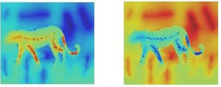
Figure.3. True color images with range of color maps

Available online:

https://edupediapublications.org/journals/index.php/IJR/

P a g e | 2635

Figure.5: extraction of binary image

Figure.6: Manually segmented images

EVALUATION METRIC

The results of evaluation of image is obtained by the proposed method and is compared with the manually segmented image.. Let us represent „M‟ be the manual segmented image and „A‟ be the segmented image.

The Similarity Index (SI), Correct Detection Ratio (CDR), Under Segmentation Error (USE) and Over

Segmentation Error (OSE) are used for efficient evaluation. SI is a measure which offers true segmented region relative to the total segmented region. CDR indicates the degree of trueness of the actual image. USE is the ratio of the number of pixels falsely identified as segmented image by the proposed method to that of manual segmented image. OSE is the ratio of number of pixels falsely identified as unsegmented image by the proposed method to that ofmanual segmented image. We define Total Segmentation Error (TSE) as the sum of USE and OSE. The evaluation metrics SI, CDR, USE and OSE are obtained by equations.

𝑆𝐼 = 2 𝑇𝑝

Available online:

https://edupediapublications.org/journals/index.php/IJR/

P a g e | 2636 𝐶𝐷𝑅 = 𝑇𝑝

𝑇𝑝 + 𝐹𝑛× 100%

𝑈𝑆𝐸 = 2𝐹𝑛

𝑇𝑝 + 𝐹𝑛× 100%

𝑂𝑆𝐸 = 𝐹𝑛

𝑇𝑝 + 𝐹𝑛× 100%

𝑇𝑆𝐸 = 𝑈𝑆𝐸 + 𝑂𝑆𝐸

Table: Evaluation metric

Inp ut 1

Inp ut 2

Similarity index(SI) 0.88

37 0.92 85 Correct detection ratio(CDR 0.88 35 0.89 17 Under segmentation error(USE) 0.11 60 0.02 89 Over segmentation error(OSE) 0.11 65 0.10 83 Total segmentation error(TSE) 0.23 25 0.13 72

CONCLUSION

We have conferred a completely unique framework supporting the subMarkov random walk for interactive seeded image segmentation in this work. This framework are often explained as a traditional random walker that walks on the graph by adding some new auxiliary nodes, that makes our framework simply interpreted and a lot of versatile. Below this framework, we unify the well-known RW-based algorithms that satisfy the subMarkov property and build bridges to create it simple to remodel the findings between them. What is more, we've got designed a novel subRW with label before solve the twigs segmentation problems by adding previous nodes into our framework. The experimental results have shown that our algorithmic outperforms the progressive

RW-based algorithms. This also proves that it's practicable to style a replacement subRW algorithmic program by adding new auxiliary nodes into our framework. We can extend our algorithmic program to a lot of applications, such as center line detection at 3D medical pictures and classification. Finally some of the parameters of an algorithm have been changed to reduce the noise of an image as well as to extract the particular region of an image with perfect edges and flexibility.

REFERENCES

[1] L.Grady,“Randomwalksforimagesegmentation, ”IEEETrans. PatternAnal.Mach.Intell., vol. 28,no. 11,pp. 1768–1783,Nov.2006.

[2] T. H. Kim, K. M. Lee, and S. U. Lee, “Generative image segmentation using random walks with restart,” in Proc. ECCV, 2008, pp. 264–275.

[3]J. Shen, Y. Du, W. Wang, and X. Li, “Lazy random walks for superpixel segmentation,” IEEE Trans. Image Process., vol. 23, no. 4, pp. 1451– 1462,Apr.2014.

[4]X.-M. Wu, Z. Li, A. M.So, J. Wright, and S.-F. Chang, “Learning with partially absorbing random walks,” in Proc. NIPS, 2012, pp. 3077–3085.

[5]A. K. Sinop and L. Grady, “A seeded image segmentation framework unifying graph cuts and random walker which yields a new algorithm,” in Proc. IEEE ICCV, Oct. 2007, pp. 1–8.

Available online:

https://edupediapublications.org/journals/index.php/IJR/

P a g e | 2637

[7]L. J. Grady and J. Polimeni, Discrete Calculus: Applied Analysis on Graphs for Computational Science. Springer, 2010.

[8] C. Couprie, L. Grady, L. Najman, and H. Talbot, “Power watershed: A unifying graph-based optimization framework,” IEEE Trans. PatternAnal. Mach. Intell., vol. 33, no. 7, pp. 1384–1399, Jul.2011.

[9] Yuri boycov,garethfunka-lea,” Graph Cuts and Efficient N-D Image Segmentation” in International Journal of Computer Vision 70(2), 109– 131,2006.

[10] N. Biggs, “Algebraic potential theory on graphs,” Bulletin of London Mathematics Society, vol. 29, pp. 641– 682,1997.

[11] L. Grady and G. Funka-Lea, “Multi-label image segmentation for medical applications based on graph-theoretic electrical potentials,” in Computer Vision and Mathematical Methods in Medical and Biomedical Image Analysis, ECCV 2004, no. LNCS3117. Prague, Czech Republic: Springer, May 2004, pp.230–245.

[12] R. Wallace, P.-W. Ong, and E. Schwartz, “Space variant image processing,” International Journal of Computer Vision, vol. 13, no. 1, pp. 71–90, Sept.1994.

[13] L. Grady, “Space-variant computer vision: A graph-theoretic approach,” Ph.D. dissertation, Boston University, Boston, MA,2004.

[14] S. Kakutani, “Markov processes and the Dirichlet problem,” Proc. Jap.Acad., vol. 21, pp. 227–233,1945.

[15]