Natural Frequency Extraction Using Generalized Pencil-of-Function Method and Transient Response Reconstruction

(1)

NATURAL FREQUENCY EXTRACTION USING GENERALIZED PENCIL-OF-FUNCTION METHOD AND TRANSIENT RESPONSE RECONSTRUCTION

J.-H. Lee

Department of Information & Communication Engineering Sejong University

98, Kunja-dong, Kwangjin-ku, Seoul, 143-747, Korea

H.-T. Kim

Department of Electronic & Electrical Engineering Pohang University of Science & Technology (POSTECH)

San 31, Hyoja-Dong, Nam-Ku, Pohang, Kyoung-buk, 790-784, Korea

Abstract—A technique for natural frequency extraction without a prior knowledge of the number of natural frequencies is proposed. The proposed scheme is based on the GPOF method with the overestimated number of natural frequencies, and it has been shown from simulation result that the proposed method is superior to the GPOF method. The method is applied to the extraction of the natural frequencies of the thin wires whose exact natural frequencies are known. While the absence of the true natural frequency has much eﬀect on the transient response reconstruction, the absence of the spurious natural frequency has little eﬀect on the transient response reconstruction. Using the above property, true natural frequencies and spurious natural frequencies can be discriminated.

1. INTRODUCTION

(2)

of scatterer. Any algorithm for the natural frequency extraction should be as noise insensitive and accurate as possible. To obtain the natural frequencies from a transient response of a target, a generalized pencil-of-function (GPOF) method is proposed by Hua et al. [7–9]. The GPOF method requires a prior knowledge of the number of natural frequencies contained in the transient data. Theoretically, the number of natural frequencies can be determined with transient data [10–13]. But in lowsignal-to-noise ratio (SNR) environment, it is diﬃcult to determine it correctly. In this study, natural frequency extraction method using the GPOF method without a prior knowledge of the number natural frequencies is considered. The number of natural frequencies is overestimated and the resulting spurious natural frequencies are discriminated from the true natural frequencies.

2. GENERALIZED PENCIL OF FUNCTION METHOD

In this section, the GPOF method is described brieﬂy [7]. Late time transient response sampled with time intervalδtcan be expressed by

yk = M

i=1

biexp(siδt k) k= 0, . . . , N−1 (1)

where si are the natural frequencies, bi are the residues, M is the

number of natural frequencies. For brevity, let us deﬁne

zi= exp(siδt). (2)

The natural frequencies can be extracted from target measurement datayk using the GPOF method. We deﬁne the matricesY1 andY2 as

Y1 = [y0, y1, . . . , yL−1] (3)

Y2 = [y1, y2, . . . , yL] (4)

where matrix element vectoryi is given by

yi = [yi, yi+1, . . . , yi+N−L−1]T. (5)

Then {zi}Mi=1 are the eigenvalues of Z.

Z =D−1UHY2V (6)

where D, U and V are given by the singular value decomposition of

Y1.

Y1 =

M

i=1

(3)

Y₁+ = V D−1UH (8)

The superscriptHdenotes the conjugate transpose of a matrix. {si}Mi=1 can be obtained from{zi}Mi=1 with (2).

3. PROCEDURE FOR EXTRACTING THE TRUE NATURAL FREQUENCIES

Let M0 be the number of the true natural frequencies which should be known a priori in the GPOF method. It is known that natural frequencies occur in complex conjugate pairs for real valued transient response. Thus, the true natural frequencies can be represented by

{si}M_i₌₁0/2 and {si∗}M_i₌₁0/2 where M0 is the number of the true natural frequencies. In the ﬁrst place,M1 andM2 which are suﬃciently larger than the expectedM0 are chosen. Note that it is not necessary to know

M0 exactly to determine M1 and M2. The GPOF method is applied with M = M1 > M0, M = M2 > M0 and the extracted natural frequencies are denoted by sa

i (i = 1,· · ·, M1), sbi (i = 1,· · ·, M2), respectively. In {sa_i}M1

i=1 and {sbi}Mi=12, there exist spurious natural frequencies because more natural frequencies than actually exist is assumed in the GPOF method. The objective is to select M0 true natural frequencies out of {sa_i}M1

i=1 and {sbi}Mi=12. As previously stated, natural frequencies occur in complex conjugate pairs. In addition to it, the real part of the natural frequencies must be negative for the physical constraint of power balance. From {sa_i}M1

i=1, the natural frequencies which do not satisfy the above requirement are excluded. The remaining natural frequencies are denoted by {sA_i , sA_i ∗}MA/2

i=1 , and the corresponding natural frequencies for {sb_i}M2

i=1 are denoted by {sB

i , sBi

∗_}MB/2

i=1 where MA and MB are the number of the

natural frequencies satisfying the above requirement for {sa_i}, {sb_i}, respectively. Here MA and MB are less than or equal to M1 and M2, respectively. Let{sc_i, sc_i∗}M3/2

1 denote the common natural frequencies of {sA

i , sAi

∗_}MA/2

i=1 and {sBi , sBi

∗_}MB/2

i=1 , where M3 is the number of common natural frequencies.

For suﬃciently largeM1and M2, the true natural frequencies will be extracted for both M1 and M2. But spurious natural frequencies extracted for M1 may not be extracted for M2. Thus, all of the true natural frequencies will belong to {sc

i, sci∗} M3/2

i=1 . But the spurious natural frequencies may or may not belong to {sc_i, sc_i∗}M3/2

i=1 . Consequently, {sc_i, sc_i∗}M3/2

(4)

frequencies. There are M3 − M0 spurious natural frequencies in

{sc i, sci∗}

M3/2

i=1 . Howto determine M0 and howto choose M0 true natural frequencies out ofM3 natural frequencies will be explained in Section 4–Section 6.

Using the method in Section 4, it can be determined whether

{sc i, sci∗}

M3/2

i=1 contains all of the true natural frequencies. If it does not include all of the true natural frequencies, this is because

M1 and M2 used for the GPOF method are too small to include all of the true natural frequencies. So we must stop and increase

M1 and M2. If it does include at least all of the true natural frequencies, the method in Section 5 is used with p = 0, m =

M3, {sˆi(m/2), sˆ∗i(m/2)} m/2

i=1= {sci, sci∗} M3/2

i=1 to check if there are spurious natural frequencies where{ˆsi(m/2), ˆs∗i(m/2)}

m/2

i=1 denotes the undetermined m natural frequencies. If there are no spurious natural frequencies,M0 =mand the true natural frequencies{si, si∗}Mi=10/2 are given by the remaining natural frequencies of{ˆsi(m/2), ˆs∗i(m/2)}

m/2

i=1. When there are spurious natural frequencies, the method in Section 6 is used. One natural frequency pair is excluded and m decreases by two. If a condition for the true natural frequencies which will be stated later is satisﬁed, the natural frequencies are selected as the true natural frequencies and excluded. Each time natural frequency pair is excluded, m decreases by two. Whenever the true natural frequency pair is excluded, p increases by two. Initial value for p is zero. Thus,

p denotes the number of the selected true natural frequencies. The

p selected true natural frequencies when there are m undetermined natural frequencies are denoted by {si(m/2), si∗(m/2)}p/_i=12. Another natural frequency pair is excluded in the same manner until there are no spurious natural frequencies. The true natural frequencies are given by the p selected natural frequencies and ﬁnally remaining natural frequencies {ˆsi(m/2), ˆs∗i(m/2)}

m/2

i=1.

4. TRANSIENT RESPONSE RECONSTRUCTION

Whether the speciﬁc natural frequencies{s¯i, s¯∗i} m/2

i=1 contains at least all of the true natural frequencies {si, s∗i}

M0/2

i=1 , can be determined using transient response reconstruction. The transient response of a scatterer with natural frequencies of {si, s∗i}

M0/2

i=1 can be represented as

yk= M0/2

i=1

biexp[siδtk] + M0/2

i=1

(5)

Given {yk}N0−1 and {¯si, s¯∗i} m/2

i=1, {¯bi, ¯b∗i} m/2

i=1 is the least squares solution of (10).

yk= m/2

i=1

¯_b_i_exp[¯_s_i_δtk_{] +}

m/2

i=1 ¯_b∗

i exp[¯s∗iδtk] k= 0, . . . , N−1 (10)

Usually the number of transient late time data N is greater than the number of natural frequencies m in (10). So (10) is an overdetermined system. Because {¯bi, ¯b∗i}

m/2

i=1 is the least squares solution, it does not exactly satisfy equations in (10).

Using the obtained {¯bi, ¯b∗i} m/2

i=1, the transient response is reconstructed [5].

y(recon)k≡ m/2

i=1

¯_b_i_exp[¯_s_i_δtk_{] +}

m/2

i=1 ¯_b∗

i exp[¯s∗iδtk] k= 0, . . . , N−1 (11)

The following factor is deﬁned withyk and y(recon)k ;

ρ= 1− N₋1

k=0[yk−y(recon)k]2

N−1

k=0[yk]2

(12)

Comparing (10) and (11), if there is no error in the least squares solution {¯bi, ¯b∗i}

m/2

i=1, y(recon)k and yk will coincide exactly and ρ is

equal to unity. But because (10) is an overdetermined system, there is an inevitable error in the least squares solution{¯bi, ¯b∗i}

m/2

i=1,y(recon)k

and yk will not coincide exactly, which means ρ can not be unity. If

{s¯i, ¯s∗i} m/2

i=1 includes {si, si∗}Mi=10/2, there will be little error and ρ is nearly unity. But if {s¯i, s¯∗i}

m/2

i=1 does not include {si, si∗}

M0/2 i=1 , there will be much error in the least squares solution andρwill be much less than 1. A threshold value of ρthreshold is chosen. If ρ > ρthreshold, it is assumed that {s¯i, ¯s∗i}

m/2

i=1 includes {si, si∗} M0/2

i=1 , Similarly if

ρ < ρthreshold, it is assumed that{¯si, s¯∗i} m/2

i=1 does not include all of the true natural frequencies.

5. HOW TO CHECK THE EXISTENCE OF SPURIOUS NATURAL FREQUENCIES

(6)

frequencies {si(m/2), si∗(m/2)}p/_i₌₁2, it can be determined whether all

of the undetermined natural frequencies {sˆi(m/2), sˆi∗(m/2)}m/i=12 are the true natural frequencies.

Let {bˆi(m/2), bˆi∗(m/2)}im/=12, {bi(m/2), bi∗(m/2)}p/i=12 denote the least squares solution of (13).

yk = m/2

i=1 ˆ

bi(m/2) exp[ ˆsi(m/2)δt k]

+

m/2

i=1 ˆ

bi

∗

(m/2) exp[ ˆsi∗(m/2)δt k]

+

p/2

i=1

bi(m/2) exp[si(m/2)δt k]

+

p/2

i=1

bi∗(m/2) exp[si∗(m/2)δt k] k= 0, . . . , N−1 (13)

Similarly,{bˆi(m/2, j), bˆi∗(m/2, j)}im/=12,{bi(m/2, j), bi∗(m/2, j)}p/i=12 is the least squares solution of (14)

yk = m/2

i=1, i=j

ˆ

bi(m/2, j) exp[ ˆsi(m/2)δt k]

+

m/2

i=1, i=j

ˆ

bi∗(m/2, j) exp[ ˆsi∗(m/2)δt k]

+

p/2

i=1

bi(m/2, j) exp[si(m/2)δt k]

+

p/2

i=1

bi∗(m/2, j) exp[si∗(m/2)δt k] k= 0, . . . , N−1 (14)

As in Section 4, the reconstructed responses are deﬁned.

y(recon)k(m/2)≡ m/2

i=1 ˆ

bi(m/2) exp[ˆsi(m/2)δt k]

+

m/2

i=1 ˆ

(7)

+

p/2

i=1

bi(m/2) exp[si(m/2)δt k]

+

p/2

i=1

bi∗(m/2)exp[si∗(m/2)δt k]k= 0, . . . , N−1 (15)

y(recon)k(m/2, j) is deﬁned by the following equations for each j= 1, . . . , m/2.

y_(recon)_k(m/2, j)≡

m/2

i=1, i=j

ˆ

bi(m/2, j) exp[ˆsi(m/2)δt k]

+

m/2

i=1, i=j

ˆ

bi∗(m/2, j) exp[ ˆsi∗(m/2)δt k]

+

p/2

i=1

bi(m/2, j) exp[si(m/2)δt k]

+

p/2

i=1

bi∗(m/2, j)exp[si∗(m/2)δtk]k= 0, . . . , N−1(16)

To discriminate the correlation factors of y(recon)k(m/2) and y(recon)k(m/2, j),ρ(m/2) andρ(m/2, j) are deﬁned.

ρ(m/2) = 1−

N₋1

k=0

[yk−y(recon)k(m/2)]2

N₋1

k=0 [yk]2

(17)

ρ(m/2, j) = 1−

N−1

k=0

[yk−y(recon)k(m/2, j)]2

N−1

k=0 [yk]2

j= 1, . . . , m/2. (18)

Note that{si(m/2), si∗(m/2)}p/i=12 denotes the selected true natu-ral frequencies when there are m undetermined natural frequencies. Thus, if {sˆi(m/2), ˆs∗i(m/2)}

m/2

i=1 are the true natural frequencies,

{si(m/2), si∗(m/2)}p/i=12 and{sˆi(m/2), sˆ∗i(m/2)} m/2

(8)

true natural frequencies. According to Section 4,ρ(m/2) is larger than

ρthreshold because {si(m/2), si∗(m/2)}ip/=12, {ˆsi(m/2), sˆ∗i(m/2)} m/2

i=1 contains all of the true natural frequencies. But ρ(m/2, j) w hich is calculated without {sˆj(m/2), sˆ∗j(m/2)} will be less than ρthreshold

because {si(m/2), si∗(m/2)} p/2

i=1, {sˆi(m/2), ˆs∗i(m/2)} m/2

i=1 without

{sˆj(m/2), ˆs∗j(m/2)} does not include all of the true natural

frequen-cies.

On the contrary, suppose there are spurious natural frequencies as well as the true natural frequencies in {sˆi(m/2), ˆs∗i(m/2)}

m/2

i=1. Even though there are spurious natural frequencies in{sˆi(m/2), sˆ∗i(m/2)}

m/2

i=1,

ρ(m/2) is greater thanρthresholdbecause there are all of the true natu-ral frequencies in{sˆi(m/2), sˆ∗i(m/2)}

m/2

i=1 and{si(m/2), si∗(m/2)}

p/2

i=1. The number of the spurious natural frequencies is m +p −M0. If

{sˆj(m/2), sˆ∗j(m/2)} is the true natural frequency, {si, si∗}p/i=12 and

{sˆi(m/2), sˆi∗(m/2)}_im/₌₁2 without{sˆj(m/2), sˆ∗j(m/2)}does not include

{si, si∗}Mi=10/2. But if ˆsj is not the true natural frequency, {si, si∗}p/i=12 and{sˆi(m/2), sˆi∗(m/2)}im/=12without{ˆsj(m/2), sˆ∗j(m/2)}does include

{si, si∗}Mi=10/2. Because of the spurious natural frequencies, there will be some j whose ρ(m/2, j) is larger than ρthreshold since transient re-sponse can be reconstructed without one spurious natural frequency pair.

6. HOW TO EXCLUDE SPURIOUS NATURAL FREQUENCY PAIR AND TRUE NATURAL FREQUENCY PAIR

As previously stated, if ρ(m/2, j) > ρthreshold for certain j, there are spurious natural frequencies in{ˆsi(m/2), sˆ∗i(m/2)}

m/2

i=1. To select true natural frequency pair and spurious natural frequency pair, the following equation is deﬁned using ˆbi(m/2), ˆbi(m/2, j), bi(m/2) and bi(m/2, j) of (13) and (14).

d(m/2, j) =

m/2

i=1,i=j

ˆ

bi(m/2)−bˆi(m/2, j)

ˆ

bi(m/2)

+ p/2 i=1

bi(m/2)−bi(m/2, j) bi(m/2)

(9)

d(m/2, j) represent the sum of the diﬀerence of the obtained least squares solution with and without ˆsj(m/2) and ˆs∗j(m/2).

Thus, large d(m/2, j) means {ˆsj(m/2), ˆs∗j(m/2)} has much

eﬀect on the least squares solution. Let jmin and jmax denote

j whose d(m/2, j) is the minimum and the maximum of all

{d(m/2, j)}m/_i₌₁2 respectively. {sˆjmin(m/2), ˆs∗jmin(m/2)} has the least

eﬀect on least squares solution and {sˆjmax(m/2), ˆs∗jmax(m/2)} has

the greatest eﬀect on least squares solution. It is assumed that

{sˆjmin(m/2), ˆs∗jmin(m/2)} is spurious natural frequency pair and is

excluded from{sˆi(m/2), sˆi∗(m/2)}m/_i₌₁2. Ifd(m/2, jmax) is much larger

than d(m/2, jmin), {ˆsjmax(m/2), sˆ∗jmax(m/2)} is considered to be the

true natural frequency pair. As a rule of thumb, whetherd(m/2, jmax)

is larger than ten timesd(m/2, jmin) or not is used as a criterion. The

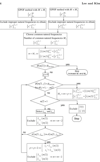
ﬂowchart for extraction of the natural frequencies is given in Fig. 1.

7. NUMERICAL RESULTS

To justify the proposed scheme for natural frequency extraction, computer simulation was performed. Scattering data were generated using a frequency-domain method-of-moments solution. A piecewise-sinusoidal basis function is employed and thin-wire approximation was used. The backscattering complex ﬁeld values were calculated at 64 and 128 equally spaced frequencies. The frequency step is 7.8 MHz. An inverse Fourier transform was subsequently applied to these results to obtain the simulated transient response. The Gaussian random noise is added to the transient response for noise simulation. Each point of the thin wire transient response is perturbed with a Gaussian noise. The signal to noise ratio is deﬁned as follows.

S/N (dB) = 10 log 1

σ2

γ−1

i=0

|yi|2

γ (20)

whereσ2is the variance of Gaussian noise and{yi}γ_i₌₀−1are the late time

transient data and γ is the number of data considered. The angular frequency range covered with 64 frequency responses and 128 frequency responses are

7.8×106×63×2π = 3.088×109 (rad) (21)

(10)

{ }

1

GPOF method with

M a i

i

M M

s =

=

{ }

2

1

GPOF method with

M b i _i

M M s

=

Exclude improper natural frequencies to obtain Exclude improper natural frequencies to obtain

3

Choose common natural frequencies Number of common natural frequencies M

(m2)< threshold

0 p=

( 2 , ) threshold

for all 1, , 2 m j

j m

< =

2 1 m =

min max

Select j and j

( 2 , max) ( 2 , min)

d m j d m j

Stop

no

yes

no no

yes

no

ρ ρ

(11)

Table 1. First ten natural frequencies pairs of thin wire(L/a= 200).

normalized unnormalized (L=1m) (×109₎

1 -0.0828 +j 0.9251 -0.07803 +j 0.8719 -0.0828 -j 0.9251 -0.07803 -j 0.8719 2 -0.1212 +j 1.912 -0.1142 +j 1.802

-0.1212 -j 1.912 -0.1142 -j 1.802 3 -0.1491 +j 2.884 -0.1405 +j 2.718

-0.1491 -j 2.884 -0.1405 -j 2.718 4 -0.1713 +j 3.874 -0.1614 +j 3.651

-0.1713 -j 3.874 -0.1614 -j 3.651 5 -0.1909 +j 4.854 -0.1799 +j 4.574

-0.1909 -j 4.854 -0.1799 -j 4.574 6 -0.2080 +j 5.845 -0.1960 +j 5.509

-0.2080 -j 5.845 -0.1960 -j 5.509 7 -0.2240 +j 6.829 -0.2111 +j 6.436

-0.2240 -j 6.829 -0.2111 -j 6.436 8 -0.2383 +j 7.821 -0.2245 +j 7.371

-0.2383 -j 7.821 -0.2245 -j 7.371 9 -0.2522 +j 8.807 -0.2376 +j 8.301

-0.2522 -j 8.807 -0.2376 -j 8.301 10 -0.2648 +j 9.800 -0.2495 +j 9.237

-0.2648 -j 9.800 -0.2495 -j 9.237

Table 1 shows the first ten natural frequencies pairs of thin wire with length/radius = 200 [1]. In Table 1, it can be seen that the imaginary part of the first three natural frequencies pairs are below 3.088 × 109(rad) and the imaginary part of the first six natural frequencies pairs are below6.224×109(rad). Thus, the first three natural frequencies pairs are contained in the simulated transient response when using 64 frequency responses, and the first six natural frequencies pairs are contained in the simulated transient response when using 128 frequency responses. From sampling theorem, the sampling interval must be not more than π/ωm apart where ωm is

(12)

pairs and 5.048× 10−10 for the extraction of the ﬁrst six natural frequencies pairs.

Using the transient response of SNR of 20 dB obtained from the 64 frequency-responses, the ﬁrst three natural frequencies pairs can be extracted. In these examples, ρthreshold of 0.9 is used and sampling interval is 4×10−10 which is in the range of 11.5×10−11. Here we choose M1 of 20 and M2 of 18. The GPOF method is applied with L = 20, M1 = 20, N = 40 and L = 20, M2 = 18,

N = 40. In this case, MA,MB, and M3 happen to be 20, 16 and 14, respectively. Fourteen common natural frequencies and the subsequent discrimination procedure is illustrated in Table 2. In Table 2, only the natural frequencies whose imaginary part is positive are shown. With

m = M3 = 14, ρ(7) is larger than ρthreshold and {ρ(7, i)}7i=1 are not less than ρthreshold for all i = 1, . . . ,7. Thus, according to Section 5, it is assumed that there are spurious natural frequencies. To exclude natural frequency pairs, {d(7, i)}7_i₌₁ are calculated and the minimum and the maximum of all {d(7, i)}7_i₌₁ are chosen. From Table 2, it is observed that d(7,3) is the minimum and d(7,1) is the maximum. ˆ

s3(7) and ˆs∗3(7) are excluded and m decreases by 2 from 14 to 12. Since d(7,1) is larger than ten times d(7,3), {sˆ1(7), ˆs∗1(7)} is selected as {s1, s1∗} and excluded. p increases by two from zero to two and

m decreases by two. With the remaining ten natural frequencies of

{sˆi(5), sˆi∗(5)}5i=1,{d(5, i)}5i=1 are calculated. Alsoρ(5) is larger than

ρthresholdand{ρ(5, i)}i5=1 are not less thanρthresholdfor alli= 1, . . . ,5, implying the existence of spurious natural frequencies. The minimum and the maximum of{d(5, i)}5

i=1 are chosen. The minimum is d(5,4) and the fourth natural frequency pair is excluded and m decreases from ten to eight. Condition for true natural frequency is satisﬁed and {ˆs1(5), ˆs∗1(5)} is selected as {s2, s2∗} and excluded. p increases from two to four and m decreases from eight to six. It is repeated until {d(m/2, i)}_im/₌₁2 are less than ρthreshold for all i = 1,· · ·, m/2. In this example,{ρ(1, i)}1

i=1 is less thanρthreshold. Thus,{sˆ1(1), ˆs∗1(1)}is the true natural frequency pair. Fig. 2 illustrates the exact natural frequencies, natural frequencies extracted using the GPOF method with L = 20, M0 = 6, N = 40 and natural frequencies extracted using our method. It is shown that the natural frequencies extracted by our method is more accurate. With the same L,M1, M2,M0 and

N, the corresponding results for SNR of 30 dB are presented in Table 3 and Fig. 3.

(13)

Table 2. Selecting true natural frequencies (SNR = 20 dB, three natural frequencies pairs).

ρ(7) 0.994938 state

i siˆ(7) ρ(7, i) d(7, i)

1 -0.0906607 +j 0.911136 0.891326 26.1098 true (s1)

2 -0.133584 +j 1.88521 0.982303 10.22956 undetermined 3 -0.0923101 +j 5.85415 0.994347 1.17856 spurious 4 -0.161559 +j 4.74416 0.993366 2.40442 undetermined 5 -0.137720 +j 3.76205 0.989987 4.58826 undetermined 6 -0.0489817 +j 3.28859 0.986676 1.19432 undetermined 7 -0.154516 +j 2.89268 0.987316 4.70505 undetermined

ρ(5) 0.994347 state

i siˆ(5) ρ(5, i) d(5, i)

1 -0.133584 +j 1.88521 0.982046 10.00019 true (s2)

2 -0.161559 +j 4.74416 0.993227 1.30021 undetermined 3 -0.137720 +j 3.76205 0.989625 4.17326 undetermined 4 -0.0489817 +j 3.28859 0.986168 0.891189 spurious 5 -0.154516 +j 2.89268 0.986575 4.66208 undetermined

ρ(3) 0.986168 state

i siˆ(3) ρ(3, i) d(3, i)

1 -0.161559 +j 4.74416 0.984985 1.04358 spurious 2 -0.137720 +j 3.76205 0.977552 2.88703 undetermined 3 -0.154516 +j 2.89268 0.973224 4.40101 undetermined

ρ(2) 0.984985 state

i siˆ(2) ρ(2, i) d(2, i)

1 -0.137720 +j 3.76205 0.975040 1.80875 spurious 2 -0.154516 +j 2.89268 0.968638 2.39563 undetermined

ρ(1) 0.975040 state

i siˆ(1) ρ(1, i) d(1, i)

1 -0.154516 +j 2.89268 0.456913 1.41963 true (s3)

natural frequencies pairs can be extracted. The results for SNR of 20 dB withM1 = 20, M2 = 18 are shown in Table 4 and Fig. 4. The GPOF methods withL= 20,M1 = 20,N = 40 and L= 20, M2= 18,

N = 40 are used. The procedure for true natural frequency selection is shown in Table 4. The conventional GPOF method is applied with

(14)

-0.2 -0.18 -0.16 -0.14 -0.12 -0. 1 -0.08 0.5

1 1.5 2 2.5 3

Re[Normalized natural frequencies]

Im[Normalized natural frequencies]

exact GPOF method Proposed method

Figure 2. Extracted natural frequencies (SNR = 20 dB, three true natural frequencies pairs).

-0.2 -0.18 -0.16 -0.14 -0.12 -0. 1 -0.08

0.5 1 1.5 2 2.5 3

(15)

Table 3. Selecting true natural frequencies (SNR = 30 dB, three true natural frequencies pairs).

ρ(5) 0.989796 state

i siˆ(5) ρ(5, i) d(5, i)

1 -0.0857292+j 0.912428 0.581495 73.9304 true (s1)

2 -0.122845 +j 1.88618 0.989253 3.86233 undetermined 3 -0.122662+j 4.77972 0.989695 1.74639 spurious 4 -0.143351+j 4.08567 0.989334 1.86280 undetermined 5 -0.146231 +j 2.87137 0.844520 66.1954 undetermined

ρ(3) 0.989695 state

i siˆ(3) ρ(3, i) d(3, i)

1 -0.122845 +j 1.88618 0.989253 21.3006 undetermined 2 -0.143351 +j 4.08567 0.989216 1.03916E-01 spurious 3 -0.146231 +j 2.87137 0.819969 32.0684 true (s2)

ρ(1) 0.989216 state

i siˆ(1) ρ(1, i) d(1, i)

1 -0.122845 +j 1.88618 0.503264 1.19583 true (s3)

-0.22 -0.2 -0.18 -0.16 -0.14 -0.12 -0. 1 -0.08

1 2 3 4 5 6

(16)

Table 4. Selecting true natural frequencies (SNR = 20 dB, six true natural frequencies pairs).

ρ(8) 0.995117 state

i siˆ(8) ρ(8, i) d(8, i)

1 -0.0864837 +j 0.899732 0.780497 6.67516 undetermined

2 -0.123205 +j 1.89848 0.710686 13.9417 undetermined 3 -0.140275 +j 2.87221 0.744482 17.4737 undetermined

4 -0.160085 +j 3.85850 0.789838 20.2802 true(s1)

7 -0.0314307 +j 6.64646 0.965921 5.57765 undetermined

8 -0.144739 +j 7.56264 0.993917 1.30921 spurious

ρ(6) 0.993917 state

i siˆ(6) ρ(6, i) d(6, i)

3 -0.140275 +j 2.87221 0.739141 9.56850 undetermined

4 -0.182086 +j 4.84443 0.846527 10.08546 true (s2)

5 -0.165811 +j 5.81579 0.891441 2.78013 undetermined

6 -0.0314307 +j 6.64646 0.960090 0.647117 spurious

ρ(4) 0.960090 state

i siˆ(4) ρ(4, i) d(4, i)

1 -0.0864837 +j 0.899732 0.742198 0.978050 true (s3)

2 -0.123205 +j 1.89848 0.663337 2.15259 true (s4)

3 -0.140275 +j 2.87221 0.686860 2.38625 true (s5)

4 -0.165811 +j 5.81579 0.838084 1.62200 true (s6)

results for SNR of 30 dB are shown in Table 5 and Fig. 5.

(17)

Table 5. Selecting true natural frequencies (SNR = 30 dB, six true natural frequencies pairs).

ρ(8) 0.999701 state

i siˆ(8) ρ(8, i) d(8, i)

1 -0.0787733 +j 0.910284 0.773537 15.8967 undetermined

2 -0.119753 +j 1.88676 0.698721 35.6887 undetermined 3 -0.147986 +j 2.86483 0.742614 45.4355 true (s1)

4 -0.169511 +j 3.84825 0.810425 44.8951 undetermined

7 -0.0185108 +j 6.64673 0.968546 18.8467 undetermined 8 -0.211369 +j 7.57315 0.999638 0.359863 spurious

ρ(6) 0.999638 state

i siˆ(6) ρ(6, i) d(6, i)

3 -0.169511 +j 3.84825 0.794539 12.0660 undetermined 4 -0.190466 +j 4.83495 0.861544 10.21415 true (s2)

5 -0.197847 +j 5.81651 0.904400 3.72376 undetermined

6 -0.0185108 +j 6.64673 0.963971 0.662052 spurious

ρ(4) 0.963971 state

i siˆ(4) ρ(4, i) d(4, i)

1 -0.0787733 +j 0.910284 0.732482 0.969457 true (s3)

2 -0.119753 +j 1.88676 0.643776 2.29281 true (s4)

3 -0.169511 +j 3.84825 0.736562 2.51375 true (s5)

4 -0.197847 +j 5.81651 0.849300 1.72013 true (s6)

(18)

-0.22 -0.2 -0.18 -0.16 -0.14 -0.12 -0. 1 -0.08 1

2 3 4 5 6

Figure 5. Extracted natural frequencies (SNR = 30 dB, six true natural frequencies pairs).

8. CONCLUSION

(19)

ACKNOWLEDGMENT

This work was supported by the Korea Research Foundation Grant funded by the Korean Government (MOEHRD) (KRF-2005-003-D00261).

REFERENCES

1. Rothwell, E. J., D. P. Nyquist, K. M. Chen, and B. Drach-man, “Radar target discrimination using the extinction-pulse tech-nique,” IEEE Trans. on Ant. and Prop., Vol. 33, 929–936, Sept. 1985.

2. Chen, K. M., D. P. Nyquist, E. J. Rothwell, L. Webb, and W. M. Sun, “Newprogress on E/S pulse technique for noncooperative target recognition,” IEEE Trans. on Ant. and Prop., Vol. 40, 829–833, July 1992.

3. Blanco, D., D. P. Ruiz, E. Alameda, and M. C. Carrion, “An asymptotically unbiased E-pulse-based scheme for radar target discrimination,” IEEE Trans. on Ant. and Prop., Vol. 52, 1348– 1350, May 2004.

4. Lee, J.-H., I.-S. Choi, and H.-T. Kim, “Natural frequency-based neural network approach to radar target recognition,” IEEE Trans. on Signal Processing, Vol. 51, 3191–3197, Dec. 2003. 5. Lee, J.-H. and H.-T. Kim, “Radar target discrimination using

transient response reconstruction,” Journal of Electromagnetic Waves and Applications, Vol. 19, 655–669, May 2005.

6. Tesche, F. M., “On the analysis of scattering and antenna problems using the singularity expansion technique,”IEEE Trans. on Ant. and Prop., Vol. 21, 53–61, Jan. 1973.

7. Hua, Y. and T. K. Sarkar, “Generalized pencil-of-function method for extracting poles of an EM system from its transient response,” IEEE Trans. on Ant. and Prop., Vol. 37, 229–234, Feb. 1989. 8. Hua, Y. and T. K. Sarkar, “Matrix pencil method for estimating

parameters of exponentially damped/undamped sinusoids in noise,” IEEE Trans. on Acoust., Speech, Signal Processing, Vol. 38, 814–824, May 1990.

9. Hua, Y., “Parameter estimation of exponentially damped sinusoids using higher order statistics and matrix pencil,” IEEE Trans. on Acoust., Speech, Signal Processing, Vol. 39, 1691–1692, Jul. 1991.

(20)

theoretic criteria,” IEEE Trans. on Acoust., Speech, Signal Processing, Vol. 33, 387–392, Apr. 1985.

11. Wax, M. and I. Ziskind, “Detection of number of coherent signals by the MDL principle,” IEEE Trans. on Acoust., Speech, Signal Processing, Vol. 37, 1190–1196, Aug. 1989.

12. Fishler, E. and H. Messer, “On the use of order statistics for improved detection of signals by the MDL criterion,”IEEE Trans. on Signal Processing, Vol. 48, 2242–2247, Aug. 2000.