Development of Fundamental Theory of Thin Impedance Vibrators
Yuriy M. Penkin, Victor A. Katrich, and Mikhail V. Nesterenko*
Abstract—In the paper, we prove two theorems relating to the theory of thin impedance vibrator radiators excited by a lumped voltage generator under rather general conditions. The first theorem proves that influence of external electrodynamic media on the vibrator current distribution is limited and can be estimated using a small natural parameter. The second theorem ascertains that there exists principal possibility to compensate influence of spatial boundaries upon current distributions on a perfectly conductive vibrator by applying to its surface complex impedance with predetermined variation along the vibrator length. Several corollaries disclose a range of the theorems application and their fundamental importance.
1. INTRODUCTION
The theory of thin vibrators is now considered as classic both for perfectly conducting [1, 2] and impedance vibrators [3–10]. The theory was outlined in a large number of well-known articles and monographs (see, e.g., references in [3]). However, this problem is still of great interest, since the vibrator structures are widely used in various devices and systems to provide the required mode of excitation. Since the problem is multivariable, an experimental optimization of devices is almost impossible, and physically adequate mathematical models are needed for compound boundary value problems, non-coordinate border of spatial domains, presence of scattering irregularities, medium inhomogeneity, etc. In any case, a key stage of modeling consists in a search of current distributions on a vibrator surface. The problem solution can be greatly simplified by selection of the basic current distribution. This choice should be done taking into account the vibrator surrounding which cannot always be done relying only on analysis of available publications. Therefore, the generalization of the theoretical results concerning the influence of surrounding media upon the current distribution on the thin impedance vibrator is an actual problem.
One approach to such generalization is based on an analytical solution of an integral equation for vibrator current using small natural parameter [7]. For example, in the monograph [11], attention was drawn to the fact that the functional effect of walls of a hollow rectangular waveguide upon the current on the linear scattering vibrator located inside the waveguide contains the proportionality factor equal to the natural small parameter of the problem. An analog situation has arisen during the analytical determination of the current on a radial impedance monopole allocated on the perfectly conducting sphere [6, 9], and on the impedance vibrator over the perfectly conducting screen of finite size [10]. The boundary problem solution for these two cases requires that the total field should be represented by waves of electric and magnetic types. This article is aimed at the generalization of the influence on a boundary value problem with arbitrary boundaries that do not possess a property of mutual transformation of electric and magnetic fields. The second theorem assets that there exists principal possibility to compensate influence of spatial boundaries upon current distributions on a perfectly
Received 1 December 2015, Accepted 24 December 2015, Scheduled 5 January 2016 * Corresponding author: Mikhail V. Nesterenko (mikhail.v.nesterenko@gmail.com).
conductive radiator by covering its surface by complex impedance material with predetermined variation along the vibrator length. The second theorem states that influence of spatial boundaries upon current distributions on a perfectly conductive vibrator can be compensated by applying complex impedance with predetermined variation along the vibrator length.
2. LEMMA FORMULATION AND PROOF
To simplify the proof of the theorems, let us consider an auxiliary lemma.
Lemma. Let a thin radiating impedance vibrator, excited by a point source is placed in an infinite homogeneous medium with material parameters (ε1, μ1). The vibrator is a segment of a circular cylinder, whose radius r and the length 2L are such that inequalities [r/(2L)] 1 and r√ε1μ1/λ 1 (λis the wavelength in free space) hold. Then the electric current on the vibrator can be represented by a power series J(s) = αJ1(s) +α2J2(s) +. . . in the small parameter α = 2 ln[r/1(2L)],|α| 1, and Jn(s) is the current approximation of the n-th order (n= 1,2. . .).
Proof. The proof is based upon the well-known solution of the integral equation for the vibrator current obtained using a small natural parameter [7]. Consider the following equation [3]
1
iωε1
graddiv +k21 S
ˆ
Ger, rJrdr =−E0 (r) +zi(r)J(r), (1)
wherezi(r) is the linear intrinsic impedance ([Ohm/m]) of the vibrator,E0 (r) is the field of extraneous sources, ˆGe(r, r) is the tensor Green’s function of the spatial domain for the electric vector potential,
k1 =k√ε1μ1,k =ω/c = 2π/λ is wave number,c ≈2.998·1010cm/s is the speed of light in vacuum. Equation (1) was obtained using boundary conditions on the vibrator surfaceS if timetdependence is
eiωt and ω is a circular frequency of a monochromatic process.
In a thin wire approximation, the electric current induced on the vibrator surface can be represented as
J(r) =esJ(s)ψ(ρ, ϕ), (2)
wherees is the unit vector directed along the vibrator axis;sis the local coordinate along the vibrator
axis; ψ(ρ, ϕ) is the function of transverse (⊥) polar coordinates, satisfying the normalization condition
⊥ψ
(ρ, ϕ)ρdρdϕ= 1. If the relations
S
ˆ
Ger, rJ(r)dr =
L
−L J(s)
π
−π
e−ik1√(s−s)2+[2rsin(ϕ/2)]2
(s−s)2+ [2rsin(ϕ/2)]2ψ(r, ϕ)rdϕds
≈
L
−L
J(s)e
−ik1√(s−s)2+r2
(s−s)2+r2ds =
L
−L
J(s)e
−ik1R(s,s)
R(s, s)
R(s,s)=√(s−s)2+r2
ds (3)
are valid [1, 3] and zi(r) = zi(s) ≡ const. The surface Equation (1) can be converted to an integral
equation with a quasi-one-dimensional kernel
d2 ds2 +k
2 1
L
−L
J(s)e−ik1R
(s,s)
R(s, s) ds
=−iωε1E0
s(s) +iωε1ziJ(s), (4)
whereE0s(s) is projection of the extraneous source field on the vibrator axis.
Let us isolate a logarithmic singularity in Equation (4) core using the method described in [1, 7]
L
−L
J(s)e
−ik1R(s,s)
R(s, s) ds
= Ω(s)J(s) + L
−L
J(s)e−ik1R(s,s)−J(s) R(s, s) ds
where
Ω(s) =
L
−L
ds
(s−s)2+r2 = Ω +γ(s). (6)
γ(s) = ln[(L+s)+ √
(L+s)2+r2] [(L−s)+√(L−s)2+r2]
4L2 is a function vanishing at the vibrator center and reaching
maxima at the vibrator ends, where the current is zero as required by the boundary conditions
J(±L) = 0 [1, 3]; Ω = 2 ln2rL is a large parameter. Then, taking into account Equation (5), Equation (4) can be converted to the following integral-differential equation with a small parameter
d2J(s)
ds2 +k 2
1J(s) =α{iωε1E0s(s) +F[s, J(s)]−iωε1ziJ(s)}. (7)
Here α=−Ω1 = 2 ln[r/1(2L)] is the small natural parameter (|α| 1), and functional
F[s, J(s)] = −dJ(s
) ds
e−ik1R(s,s) R(s, s)
L −L +
d2J(s)
ds2 +k 2 1J(s)
γ(s)
+
L
−L
d2J(s)
ds2 +k 2 1J(s)
e−ik1R(s,s)−
d2J(s)
ds2 +k 2 1J(s)
R(s, s) ds
(8)
presents the vibrator eigenfield.
If we denote ˜k=k11 +iαωε1zi/k1 =k11 +i2αZ¯S/(μ1kr) ( ¯ZS =ZS/Z0 is distributed surface
impedance normalized to the wave resistance Z0 = 120π [Ohm]), Equation (7) can be written as
d2J(s)
ds2 + ˜k 2
J(s) =α{iωε1E0s(s) +F[s, J(s)]}. (9)
Since Equation (9) is proportional to the small parameterα, its solution can be obtained by a successive approximation technique using the following algorithm
⎧ ⎪ ⎪ ⎪ ⎪ ⎪ ⎪ ⎪ ⎪ ⎪ ⎨ ⎪ ⎪ ⎪ ⎪ ⎪ ⎪ ⎪ ⎪ ⎪ ⎩
d2J1(s)
ds2 + ˜k 2
J1(s) =iωε1E0s(s), d2J2(s)
ds2 + ˜k
2J2(s) =F[s, J1(s)],
· ·
d2Jn(s) ds2 + ˜k
2
Jn(s) =F[s, Jn−1(s)].
(10)
The solution of each differential equation can be obtained using the boundary conditions for the current
J1(±L) = J2(±L) = . . .=Jn(±L) = 0. Thus, we obtain the current decomposition as power series in
small parameter α, i.e.,J(s) =αJ1(s) +α2J2(s) +. . ., which was to be proved.
The zero approximation for the currentJ0 was not included into the equation system (10), since its solution is J0(s) = C1cos ˜ks+C2sin ˜ks. Taking into account losses in the medium and/or on the vibrator surface, the trigonometric functions in the solution are complex and cannot be zero for any arguments. Therefore, to satisfy the boundary conditionsJ0(±L) = 0, the constantsC1 and C2 should be zero and identitiesJ0 ≡0,F[s, J0(s)]≡0 become valid for any vibrator length.
The first approximation of the vibrator current obtained from (10) as sum of the general and partial solutions is
J(s)≈αJ1(s) =−αiωε1/˜k
sin 2˜kL ×
⎧ ⎪ ⎪ ⎪ ⎪ ⎪ ⎪ ⎨ ⎪ ⎪ ⎪ ⎪ ⎪ ⎪ ⎩
sin ˜k(L−s)
s
−L
E0sssin ˜kL+sds
+ sin ˜k(L+s)
L
s
E0sssin ˜kL−sds,
and it does not depend on the functionF[s, J(s)] (8).
3. FORMULATION AND PROOF OF THE FIRST THEOREM
Theorem 1. Let a thin radiating impedance vibrator, exited by a point source, be placed in an electrodynamic volume filled by homogeneous medium with material parameters (ε1, μ1). The volume boundary is an arbitrary Lyapunov surface S [12], not passing through sources of extraneous currents. The vibrator is a segment of a circular cylinder, whose radius r and the length 2L are such that inequalities [r/(2L)] 1 and r√ε1μ1/λ 1 (λ is the wavelength in free space) hold. Then the influence of the volume boundaries upon the current distribution on the vibrator surface does not exceed an amount proportional to the small natural parameter α= 2 ln[r/1(2L)].
Proof.The kernel ˆGe(r, r) of integral Equation (1) is the electric tensor Green’s function of the closed volume. In a system of orthogonal curvilinear coordinates (q1, q2, q3), this function, according to the general properties [12], satisfies the inhomogeneous Helmholtz equation
Δ ˆGq, q+k21Gˆ
q, q=−4πIˆδ(q1−q
1)δ(q2−q2)δ(q3−q3)
h1h2h3 , (12)
where ˆI is unit tensor; (q1, q2, q3) are source coordinates;δ(q−q) is Dirac delta function;hn are Lame
coefficients. Laplacian Δ applies to all tensor components. Then, the solution for the vector Hertz potential can be written as
Πe(q) = 1
iωε1
V
JqGˆeq, qdv+
S
divΠeqGˆeq, qn−div ˆGeq, qΠeqn
+
n,Gˆeq, qrotΠeq−
n, Πeqrot ˆGeq, q ds, (13)
wheren is the unit vector of the external normal to the surface S. The volume integral is taken over the entire volume V (dv is volume element), and the surface integral is taken over the entire surface (ds is the area element in the primed coordinates). The expression in the curly brackets is a vector, and differentiation is performed over the primed coordinates.
Thus, the solution of the inhomogeneous Helmholtz equation is the sum of the volume and surface integrals. The surface integrals can be eliminated by building the Green’s function in a special way. If the components of the Green’s function ˆGe(q, q) and components of the vector potentialsΠe(q) satisfy the boundary conditions on the surfaceS, the surface integrals vanish, since integrand of surface integrals in (13) vanish. Otherwise, the solution will have the general form (13). Thus, the expression (13) allows us to use alternative forms of the Green’s function.
If the Green’s tensor for unbounded domain, which is the solution of Equation (12) satisfying the boundary conditions at infinity is
ˆ
Ge(r, r) = ˆIe
−ik1|r−r|
|r−r| = ˆIG e
0(r, r), (14)
the vector Hertz potential (13) can be presented as
Πe(r) = 1
iωε1
V
JrIˆe
−ik1|r−r|
|r−r| dv+
S
divΠer IGˆ e0(r, r)
n−div
ˆ
IGe0(r, r)
Πern
+
n,
ˆ
IGe0(r, r)
rotΠer−
n, Πerrot
ˆ
IGe0(r, r) ds. (15)
into Equation (1), we obtain 1
iωε1
grad div +k12 S
ˆ
Ie
−ik1|r−r|
|r−r|
J(r)dr
= −E0 (r) +zi(r)J(r)−grad div +k21 S
divΠer IGˆ e0(r, r)
n−div
ˆ
IGe0(r, r)
Πern
+
n,
ˆ
IGe0(r, r)
rotΠer−
n, Πerrot
ˆ
IGe0(r, r) ds. (16)
The functional defining the field of arbitrary boundaries at the observation pointr can be found, using the relation (16)
FS
r, J(r)
= grad div +k21 S
divΠer IGˆ e0(r, r)
n
−div
ˆ
IGe0(r, r)
Πern+
n,
ˆ
IGe0(r, r)
rotΠer
−n, Πerrot
ˆ
IGe0(r, r) ds, (17)
Then, Equation (4) for the current on the vibrator surface can be written as follows
d2 ds2 +k
2 1
L
−L
J(s)e
−ik1R(s,s)
R(s, s) ds
=−iωε1E0
s(s)−iωε1FS(s, J(s)) +iωε1ziJ(s), (18)
FS(s, J(s)) is the projection of the vector functionalFS(r, J(r)) on the vibrator axis. Then, combining field functionals fΣ(r, J(r)) = F(r, J(r)) +iωε1FS(r, J(r)), in equation similar to (7), we can use the
Lemma to proof the Theorem 1. Indeed, according to Lemma, the electric current on a thin impedance vibrator can be represented by a series in the small parameter α, therefore, its first approximation, determined by the expression (11), does not depend on the functional of the boundary influence. The influence is taken into account by successive approximations. Thus, the influence of the volume boundaries on the current distribution on the vibrator does not exceed an amount proportional to the small parameter α. The Theorem 1 is proved.
3.1. Corollaries from Theorem 1
Theorem 1 is formulated for sufficiently general conditions allowing to establish several corollaries of physical interest, which define the fundamental nature of the theorem.
Corollary 1.1. Since no restrictions were imposed on magnitude of the vibrator constant impedance, the theorem is valid for a perfectly conducting vibrator, zi = 0.
Corollary 1.2. Since no restrictions were imposed on the material parameter of the medium (ε1, μ1) the theorem is valid both for unbounded space and hollow closed volumes with ε1 =μ1 = 1.
Corollary 1.3. Since the formulation and proof of the theorem does not require specifying the coordinates of a feed points0 of the voltage δ-generator E0s(s) =V0δ(s−s0), the theorem is valid for arbitrary choice of the feed point. HereV0 is the voltage amplitude,δ(s−s0) is one-dimensional Dirac delta function.
Commentary. Really, the expression for the first approximation of the current (11) was obtained for an arbitrary extraneous excitation field E0s(s). The term “arbitrary” applies only to the choice of
the feed point coordinates and model describing the local excitation source. It is related to the fact that the vibrator excitation by the incident extraneous field, formed in the spatial domain with account of the borders, which influence through structure of the field E0s(s) will have an indirect reflection in
Corollary 1.4. One of the Theorem 1 conditions are the following requirements on the surface: 1) it must be a Lyapunov surface; 2) it should not cross current sources; 3) in a more general sense, it has to be passive, i.e., without generation of extraneous fields, and 4) it does not possess the properties of mutual transformation of spatial harmonics of the electric and magnetic fields. Since the type of electrodynamic boundary surfaces is not defined and do not exclude the possibility of its composite presentation, the theorem is valid both for different types of surfaces such as perfectly conducting, impedance, partially impedance, etc. and for the different scattering inhomogeneities in the spatial domain, whose surfaces can be interpreted as parts of the total surface.
Commentary. Parts of the boundary surface can be presented by impedance surfaces of coupling holes between coupling volumes. Separate areas of piecewise inhomogeneous of the magneto-dielectric filling of the electrodynamic volume can be thought as scattering irregularities.
The approach used to the proof of Theorem 1 allows us to formulate the second theorem. It concerns the fundamental possibility to compensate the influence of the spatial boundaries upon the current distribution on a perfectly conducting vibrator using “application” of the distributed impedance on the surface.
4. FORMULATION AND PROOF OF THE SECOND THEOREM
In the proof of the Lemma and Theorem 1, linear impedance of the vibrator was assumed to be constant
zi(r) = zi(s) ≡const. Now, let us assume that the impedance can be distributed along the vibrator axiszi(r) =zi(s), or be concentrated at some points on the vibrator axis, or be superposition of these two options.
Theorem 2. Let a thin radiating impedance vibrator, exited by a point source, be placed in an electrodynamic volume filled by homogeneous medium with material parameters (ε1, μ1). The volume boundary is an arbitrary Lyapunov surface S [12], not passing through sources of extraneous currents. The vibrator is a segment of a circular cylinder, whose radius r and the length 2L are such that inequalities [r/(2L)]1and r√ε1μ1/λ1 (λisthe wavelength in free space) hold. Then, the influence of the volume boundaries upon the current distribution on the vibrator surface can be compensated by coating its surface with the complex impedance, varying along the vibrator axis, zi(s) = FS(Js,J(s)(s)). J(s) is the current distribution on the perfectly conducting vibrator, and FS(s, J(s)) is the functional (17) defining the boundary influence.
Proof. Let us consider the equation similar to Eq. (18)
d2 ds2 +k
2 1
L
−L
J(s)e
−ik1R(s,s)
R(s, s) ds
=−iωε1[E0
s(s) +FS(s, J(s))−zi(s)J(s)], (19)
where zi(s) is complex surface impedance which varies along the vibrator axis. If the equality FS(s, J(s)) =zi(s)J(s) on the right hand side of Equation (19) holds, the vibrator current is determined
only by the fields of extraneous sources. Hence, Equation (19) can be formally represented as a system of two equations ⎧
⎪ ⎪ ⎨ ⎪ ⎪ ⎩
d2 ds2 +k
2 1
L
−L J(s)e
−ik1R(s,s)
R(s, s) ds
=−iωε1E0 s(s),
FS(s, J(s))−zi(s)J(s) = 0.
(20)
The first equation is Equation (4) for a perfectly conducting vibrator, zi = 0, located in an infinite
homogeneous medium. The second equation is the functional equation, which can be solved using the current found from the first equation. These equations can be used to obtain the distribution of variable complex impedance along the vibrator axis
zi(s) = FS(s, J(s))
J(s) , (21)
wherezi(s) can be a generalized function. Thus, the influence of the boundaries can be fully compensated
impedance vibrator corresponds now to that of perfectly conducting vibrator, located in an infinite homogeneous medium with material parameters (ε1, μ1). Thus, Theorem 2 is proved.
4.1. Corollaries from Theorem 2
Corollary 2.1. Since the surface of the scattering irregularities, located in electrodynamic volume, can be interpreted as components of the common surfaceS, and the Theorem 2 is valid for this case.
Commentary. The main difficulty of the Theorem 2 application concerns determination of the functionalFS(s, J(s)). However, if Green’s function of the electromagnetic volume is known, the problem
is greatly simplified, since the fields at the boundary surfaceSin Eq. (17) can be found using the Green’s function.
Corollary 2.2. Input resistance of the impedance vibrator with the distribution in Eq. (21), positioned in the electrodynamic volume, is equivalent to that of perfectly conductive vibrator of the same geometry located in free space.
4.2. Example of Theorem 2 Application
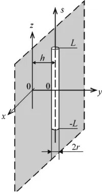
The application of the Theorem 2 can be demonstrated by the problem of the electro-magnetic radiation by a horizontal vibrator in a semi-infinite material medium [3]. Geometry of the structure and notation are shown in Fig. 1. Here {x, y, z} is a Cartesian coordinate system associated with a perfectly conducting plane, a cylindrical vibrator allocated in a medium at a distance h from the plane with material parameters (ε1,μ1). The vibrator length is 2L and its radius isr.
Figure 1. The geometry of the vibrator structure. Let us substitute Green’s function for the half-space
Gs(s, s) = e
−ik1√(s−s)2+r2
(s−s)2+r2 −
e−ik1√(s−s)2+(2h+r)2
(s−s)2+ (2h+r)2. (22)
in Equation (4). Then the equation for the vibrator current can be written as
d2 ds2 +k
2 1
L
−L
J(s)e
−ik1√(s−s)2+r2
(s−s)2+r2ds
= −iωε1E0s(s) +
d2 ds2 +k
2 1
L
−L
J(s) e
−ik1√(s−s)2+(2h+r)2
(s−s)2+ (2h+r)2ds
+iωε1z
Without loss of generality, we assume that the vibrator is excited at the center of a lumped voltage generator with an amplitudeV0. Let us apply the Theorem 2. First, we find the vibrator current in the infinite material medium by solving the first equation of the system (20) using the averaging method. The solution [3, 4, 7] is
J(s) =−αV0
iωε1
2k1
sink1(L− |s|) +αPδs(k1r, k1s)
cosk1L+αPLs(k1r, k1L) . (24)
HerePδs(k1r, k1s) =Ps[k1r, k1(L+s)]−(sink1s+ sink1|s|)PLs(k1r, k1L), the constantsPs[k1r, k1(L+s)] and PLs(k1r, k1L) are defined by the analytical formulas [3, 4, 7].
Then, substituting the currentJ(s) from (24) into the formula (21), we obtain
zi(s) =
d2 ds2 +k
2 1
L
−L
sink1(L− |s|) +αPδs(k1r, k1s) e
−ik1√(s−s)2+(2h+r)2
(s−s)2+ (2h+r)2ds
sink1(L− |s|) +αPδs(k1r, k1s) . (25) Thus, the functionalFS(r, J(r)) in (17), wherein the integration is done over an infinite boundary surface, is replaced by the functional, wherein integration is performed only over the surface of the mirror vibrator image. Since the kernel of the integral operator is a smooth function, the differentiation operator can be moved under the integral sign. The final expression for the impedance distribution function can be written as
zi(s) = F i1(s) L
−L
F isF es, sds, (26)
were
F i(s) = sink1(L− |s|) +αPδs(k1r, k1s), R1s, s=(s−s)2+ (2h+r)2,
F es, s = e−ik1R1
(s,s)
(R1(s, s))4
⎡ ⎢ ⎣
s−s2
3ik1− k 2 1−3 R1(s, s)
−R1(s, s)−ik1(R1(s, s))2+k12(R1(s, s)) 3
⎤ ⎥ ⎦.
As might be expected, ifh→ ∞in expression (26),|zi(s)| →0 for the any point on the vibrator surface.
5. CONCLUSION
The paper presents a generalization of the theory of thin impedance vibrators which can be found in a number of publications devoted to vibrator radiators with a lumped excitation in free space or in electrodynamic volumes with coordinate boundaries. Taking into account methodological aspects of the problem, the authors decided to make such a generalization in the form of two theorems. On the one hand, the approach allows systematically assessing already known results, and, on the other hand, extend the methodology to the solutions of new boundary value problems with compound surface boundaries. Requirements for the boundary surface are as follows: it must be a Lyapunov surface, which does not cross current sources, or in a more general sense, it has to be passive and does not possess the properties of mutual transformation of spatial harmonics of the electric and magnetic fields.
The first theorem proves the limited influence of the external electrodynamic medium upon the current distribution on the radiating vibrator. Quantification of this effect was related to the natural small parameter α = 2 ln[r/1(2L)]; therefore, the result would not exceed the small parameters α. The theorem proof is based on the lemma, which has independent significance. Four corollaries disclose more fully the theorems’ scope. The theorem can be used for selection of the current distribution in the vibrator for the solution of complicated boundary value problems and assessing the accuracy of this approximation.
compensated by “applying” an extended complex impedance having the required distribution to the vibrator surface. The theorems’ application was demonstrated by solving the problem for the horizontal vibrator located above a perfectly conducting plane.
The results presented in the paper can be useful both for electromagnetic theory of thin impedance vibrators and for solution of boundary value problems with vibrator excitations including the questions related physical interpretation of mathematical modeling results.
REFERENCES
1. King, R. W. P., The Theory of Linear Antennas, Harv. Univ. Press, Cambr., MA, 1956. 2. Weiner, M. M.,Monopole Antennas, Marcel Dekker, New York, 2003.
3. Nesterenko, M. V., V. A. Katrich, Yu. M. Penkin, V. M. Dakhov, and S. L. Berdnik,Thin Impedance Vibrators, Theory and Applications, Springer Science+Business Media, New York, 2011.
4. Nesterenko, M. V., “The electomagnetic wave radiation from a thin impedance dipole in a lossy homogeneous isotropic medium,” Telecommunications and Radio Engineering, Vol. 61, 840–853, 2004.
5. Nesterenko, M. V., V. A. Katrich, V. M. Dakhov, and S. L. Berdnik, “Impedance vibrator with arbitrary point of excitation,” Progress In Electromagnetics Research B, Vol. 5, 275–290, 2008. 6. Nesterenko, M. V., D. Yu. Penkin, V. A. Katrich, and V. M. Dakhov, “Equation solution
for the current in radial impedance monopole on the perfectly conducting sphere,” Progress In Electromagnetics Research B, Vol. 19, 95–114, 2010.
7. Nesterenko, M. V., “Analytical methods in the theory of thin impedance vibrators,” Progress In Electromagnetics Research B, Vol. 21, 299–328, 2010.
8. Nesterenko, M. V., V. A. Katrich, S. L. Berdnik, Y. M. Penkin, and V. M. Dakhov, “Application of the generalized method of induced EMF for investigation of characteristics of thin impedance vibrators,”Progress In Electromagnetics Research B, Vol. 26, 149–178, 2010.
9. Penkin, D. Y., V. A. Katrich, Y. . Penkin, M. V. Nesterenko, V. M. Dakhov, and S. L. Berdnik, “Electrodynamic characteristics of a radial impedance vibrator on a conduction sphere,”Progress In Electromagnetics Research B, Vol. 62, 137–151, 2015.
10. Yeliseyeva, N. P., S. L. Berdnik, V. A. Katrich, and M. V. Nesterenko, “Electrodynamic characteristics of horizontal impedance vibrator located over a finite-dimensional perfectly conducting screen,” Progress In Electromagnetics Research B, Vol. 63, 275–288, 2015.
11. Khizhnyak, N. A., Integral Equations of Macroscopical Electrodynamics, Naukova Dumka, Kiev, 1986 (in Russian).