Unconditional Stability Analysis of the 3D-Radial Point Interpolation Method and Crank-Nicolson Scheme

Unconditional Stability Analysis of the 3D-Radial Point

Interpolation Method and Crank-Nicolson Scheme

Hichem Naamen* and Taoufik Aguili

Abstract—This paper provides the theoretical validation of the unconditional stability using the Von Neumann method for the radial point interpolation method (RPIM) and Crank-Nicolson (CN) scheme, in a three dimensional (3D) problem. Moreover, the matrix inversion process, typical of the CN implicit scheme, is circumvented and approximated by a finite series for a particular stability factor range. To validate numerically the efficiency of the CN-RPIM unconditional stability, the resonant frequency inside a 2D double ridged rectangular cavity is simulated. The numerical results confirm that the CN-RPIM is significantly efficient, since the simulation time is reduced by up to 90%, and the memory requirement is saved up to 81%, with a little loss of accuracy.

1. INTRODUCTION

Well posed electromagnetic problems [1] are characteristically reduced to a set of partial differential equations (PDEs) in microwave engineering simulation and design [2]. The classical mesh-methods, such as the finite element method (FEM), method of moments (MoM) and finite difference time-domain method (FDTD), have thus been developed to convert such PDEs into sets of solvable algebraic equations [3]. Despite their wide performances the involved mesh/grid and the generated polygonisation for complex geometries [4] reduce their applications

Meshless methods use a set of unconnected nodes, randomly spread or regularly distributed to approximate the solution [5]. Among them the smoothed particle electromagnetic method (SPEM) [6], the partition of unity method (PUM) [7, 8], and the meshless local PetrovGalerkin method (MLPGM) [9] have been implemented to solve electromagnetic problems. The radial point interpolation method (RPIM) is a truly meshless method used for space discretization conjointly to the leapfrog explicit time stepping [10]. However, the Courant-Friedrich-Levy (CFL) condition limits the maximum time-step and therefore the minimal space discretization interval. To overcome such a restriction unconditionally-stable RPI methods have been elaborated centered on the implicit finite difference, such as alternating-direction implicit (ADI) and Crank-Nicolson (CN) schemes. Thus [11, 13] introduced the hybridization of the ADIRPIM and gave the proof of its unconditional stability for a three-dimensional domain. [12] proposed the CN-RPIM and numerically verified its unconditional stability for a 2-D domain as far as the locally one-dimensional RPIM (LODRPIM) [13] schemes have also been studied.

In this paper, using the Von-Neumann method based on spatial Fourier modes and for a three-dimensional open domain filled with a linear, isotropic and non-dispersive lossless medium, we theoretically justify the unconditional stability of the CN-RPIM. Moreover, the matrix inversion succeeding the Crank-Nicolson implicit scheme is theoretically approximated and numerically justified, as long as the stability factor S is inferior to 2.525 for our studied structure. The CN-RPIM is implemented for a double-ridged rectangular cavity [14, 15], and we found an excellent agreement between the numerical and analytical resonant frequencies [16] for different numerical stability factors.

Received 2 October 2017, Accepted 18 March 2018, Scheduled 10 May 2018

* Corresponding author: Naamen Hichem ([email protected]).

The memory requirements and CPU time are investigated for the CN-RPIM. The CN scheme saves up to 81% of memory and 90% of CPU time when the stability factor S= 10.

2. RADIAL POINT INTERPOLATION METHOD RPIM ALGORITHM

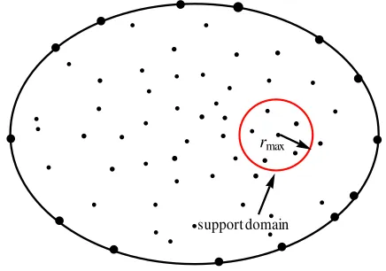
Letu(X) be a function defined in the problem domain. The RPIM interpolates u(X) around a certain nodeX(x, y, z). We force the interpolation function to pass through the function values at each scattered node, within the defined support domain shown in Figure 1. The RPIM with polynomial basis functions defines the field variable function in the following way and therefore can be written as:

u(X) =

i=N

i=1

R_i(X)a_i+

j=M

j=1

P_j(X)b_j, (1)

whereR_i(X) andP_j(X) are the radial basis functions and the polynomial basis functions, respectively;

a_iandb_j are constant coefficients yet to be determined;N is the number of nodes in the support domain controlling the number of basis functions; M is the number of polynomial basis terms. The Gaussian function is selected to be the radial basis function and defined as an exponential function of the distance

r with shape parameterc to control the decaying degree. With this choice the radial basis function is expressed as:

r_n(X) =exp

−c|r/rmax|2

, (2)

where r =

(x−x_n)2+ (y−y_n)2+ (z−z_n)2 is the distance between the point of interest X and a node atX_n(x_n, y_n, z_n) in the support domain, and rmaxis the maximum distance between the selected point to be interpolated and the nodes in the support domain. Usually the number M of polynomial basis terms is greater than the radial basis ones. Thus four terms of linear monomial basis functions are used, and the polynomial basis is [1, x, y, z]. Consequently, for the point X, Equation (1) is rewritten in the vector form as follows:

u(X) =RT(X)a+PT(X)b, (3)

where aand b are the coefficient vectors; RT(X) is the radial basis vector; PT(X) is the polynomial basis one defined as:

RT(X) = [r1(X), r2(X), r3(X), . . . , rN(X)], (4)

PT(X) = [p1(X), p2(X), p3(X), p4(X)] = [1, x, y, z]. (5) By imposing tou(X) interpolated by Equation (1) to pass throughout every scattered node in the field’s support domain of the point of interest X, an algebraic linear system is obtained relating the

rmax

support domain

factual values of field variables at the N nodes in the support domain to the unknown interpolation coefficients. The linear algebraic system expressed as a matrix equation is given by:

U_s=R₀a+P₀b, (6)

whereU_s is the vector that collects the values of field variables,R₀ the moment matrix assembling the radial basis R(X), and P₀ the moment matrix assembling the polynomial basis P(X), respectively evaluated at the N nodes in the support domain. The polynomial term of the basis function must support an additional condition that ensures a unique solution formulated as a set of homogeneous equations [5]. Henceforth, a condition of the following form is obtained:

PT₀ ·a=0. (7)

Combining Equations (6) and (7) and rewriting them in the matrix form yields:

R₀ P₀ PT₀ 0

a b

=

U_s 0

or G

a b

=

U_s 0

. (8)

R₀is anN×N moment matrix, andP₀ is anN×M matrix. SinceR₀ is symmetric, matrixGwill be symmetric too. If Gis invertible, the corresponding solution is unique for vectors of interpolationa

and b. By exploiting the nonsingular property of matrix R₀ we obtain:

b = S_bU_s, where : S_b=PT₀R−₀1P₀ −1PT₀R−₀1 (9)

a = S_aU_s, where : S_a=R₀−1−R−₀1P₀S_b. (10) Finally, the interpolation Equation (1) is rewritten:

u(X) =RT(X)S_a+PT(X)S_b U_s=Φ(X)U_s. (11) HereΦ(X) is the matrix of shape functions including N shape functions:

Φ(X) =RT(X)S_a+PT(X)S_b= [φ1(X), φ2(X), . . . φi(X), . . . φN(X)], (12) withφ_k(X) being thekth node shape function in the support domain expressed as:

φ_k(X) =

N

i=1

R_i(X)S_ika +

M

j=1

P_j(X)S_jkb . (13)

HereS_ika andS_jkb are the (ik) element and (jk) element of the constant matrices, respectively. Thus, the shape functions derivatives are deduced directly, and with q =x, y, z we find:

∂∅_k

∂q (X) =

N

i=1

∂R_i ∂q (X)S

a ik+

M

j=1

∂P_j ∂q (X)S

b

jk. (14)

Since the radial basis function has a Gaussian form, the first derivative in Equation (14) is thoroughly calculated, giving:

∂R_i

∂q (X) =−

2c r2

max

(q−q_i)R_i(x, y, z). (15)

3. IMPLEMENTATION OF THE CRANK-NICOLSON SCHEME IN THE RPIM

3.1. The 3D-RPIM Approach for Electromagnetics in Time-Domain

functions and their associated derivatives are approximated respectively by Equations (13) and (14). Thus, the RPIM algorithm is implemented in the discretized Maxwell’s equations, and the following equations are obtained:

Hn+1/2

x,i = Hnx,i−1/2+Δ_μt

⎛ ⎝

j

εn_y,j∂∅

ε j

∂z

X_iH−

j

εn_z,j∂∅

ε j

∂y

X_iH

⎞

⎠, (16)

Hn+1/2

y,i = Hny,i−1/2+

Δt μ

⎛ ⎝

j

εn_z,j∂∅

ε j

∂x

X_iH−

j

εn_x,j∂∅

ε j

∂z

X_iH

⎞

⎠, (17)

Hn+1/2

z,i = Hnz,i−1/2+

Δt μ

⎛ ⎝

j

εn_x,j∂∅

ε j

∂y

X_iH−

j

εn_y,j∂∅

ε j

∂x

X_iH

⎞

⎠ (18)

εn_x,i+1 = εn_x,i+Δt

ε

⎛ ⎝

j

Hn+1/2

z,j

∂∅H_j ∂y

X_iE−

j

Hn+1/2

y,j

∂∅H_j ∂z

X_iE

⎞

⎠ (19)

εn_y,i+1 = εn_y,i+Δt

ε

⎛ ⎝

j

Hn+1/2

x,j

∂∅H_j ∂z

X_iE−

j

Hn+1/2

z,j

∂∅H_j ∂x

X_iE

⎞

⎠ (20)

εn_z,i+1 = εn_z,i+ Δt

ε

⎛ ⎝

j

Hn+1/2

y,j

∂∅H_j ∂x

X_iE−

j

Hn+1/2

x,j

∂∅H_j ∂y

X_iE

⎞

⎠ (21)

Here, ε=ε0εr and μ=μ0μr denote the permittivity and permeability of media, respectively. ε0 and μ0 are the free space permittivity and permeability, respectively, and εr and μr are the relative permittivity and permeability, respectively. En_u,i+1 and H_u,in+1/2 are the electric and magnetic field intensities, respectively, withu=x, y, orz. Δtis the time-step increment, andX_iH is the point located at the H-node in which the spatial derivative shape functions of the neighboring E-nodes located in the selected support domain are evaluated, and the superscriptnis a temporal index. The electric and magnetic dual node distributions are staggered in space and staggered in time by one half time step.

3.2. The Crank-Nicolson Scheme Implementation in the 3D-RPIM

It was reported and confirmed in [17] that the (ADI) is systemically an approximation of the CN scheme and can also be seen as a second order perturbation of it. The Crank-Nicolson (CN) scheme solves the discretized Maxwell’s equations by a full time-step size with one marching procedure and takes the average of a forward difference and a backward difference in space in the right hand-sides of the discretized Maxwell’s equations for one full update cycle from time-step n to step n+ 1. In the time-domain, however, the electric and magnetic fields are computed not in the leap-frog way but simultaneously at the same time point in the same treated space for the structure under study. The CN scheme is applied to Equations (16), . . . , (21) which become:

εn_x,i+1X_iE = εn_x,iX_iE+Δt 2ε

⎛ ⎝

j

Hn+1

z,j

∂∅H_j ∂y

X_iE+

j

Hn_z,j∂∅Hj ∂y

X_iE

⎞ ⎠

−Δt

2ε

⎛ ⎝

j

Hn+1

y,j

∂∅H j

∂z

X_iE+

j

Hn_y,j∂∅Hj ∂z

X_iE

⎞

εn_y,i+1X_iE = εn_y,iX_iE+Δt 2ε

⎛ ⎝

j

Hn+1

x,j

∂∅H_j ∂z

X_iE+

j

Hn x,j

∂∅H_j ∂z

X_iE

⎞ ⎠

−Δt

2ε

⎛ ⎝

j

Hn+1

z,j

∂∅H_j ∂x

X_iE+

j

Hn_z,j∂∅Hj ∂x

X_iE

⎞

⎠ (23)

εn_z,i+1X_iE = εn_z,iX_iE+Δt 2ε

⎛ ⎝

j

Hn+1

y,j

∂∅H_j ∂x

X_iE+

j

Hn_y,j∂∅Hj ∂x

X_iE

⎞ ⎠

−Δt

2ε

⎛ ⎝

j

Hn+1

x,j

∂∅H_j ∂y

X_iE+

j

Hn x,j

∂∅H_j ∂y

X_iE

⎞

⎠ (24)

Hn+1

x,i

X_iH = H_x,in X_iH+Δt 2μ

⎛ ⎝

j

εn_y,j+1∂∅

ε j

∂z

X_iH+

j

εn_y,j∂∅

ε j

∂z

X_iH

⎞ ⎠

−Δt

2μ

⎛ ⎝

j

εn_z,j+1∂∅

ε j

∂y

X_iH+

j

εn_z,j∂∅

ε j

∂y

X_iH

⎞

⎠ (25)

Hn+1

y,i

X_iH = Hn_y,iX_iH+Δt 2μ

⎛ ⎝

j

εn_z,j+1∂∅

ε j

∂x

X_iH+

j

εn_z,j∂∅

ε j

∂x

X_iH

⎞ ⎠

−Δt

2μ

⎛ ⎝

j

εn_x,j+1∂∅

ε j

∂z

X_iH+

j

εn_x,j∂∅

ε j

∂z

X_iH

⎞

⎠ (26)

Hn+1

z,i

X_iH = Hn_z,iX_iH+Δt 2μ

⎛ ⎝

j

εn_x,j+1∂∅

ε j

∂y

X_iH+

j

εn_x,j∂∅

ε j

∂y

X_iH

⎞ ⎠

−Δt

2μ

⎛ ⎝

j

εn_y,j+1∂∅

ε j

∂x

X_iH+

j

εn_y,j∂∅

ε j

∂x

X_iH

⎞

⎠ (27)

These equations remain unchanged even for a domain excited with a source.

4. STABILITY ANALYSIS OF THE CN-RPIM

The Von-Neumann method is used to analyze the stability of the CN-RPIM. The instantaneous values of the electric and magnetic fields are Fourier transformed into the spatial spectral domain, for each time-stepn. Consider an open domain uniformly discretized with dual staggered grids, an electric and a magnetic ones, which are spread respectively along theE-nodes andH-nodes. EveryE-node is enclosed by eight H-nodes, and vice versa. The computation of the spatial derivatives shape functions and the fields phasors calculus are reported in the appendix. For a linear isotropic homogeneous lossless media in Cartesian coordinates and applying the discrete Fourier transform to Equations (22)–(27) yields the following ones:

εn_x+1 = εn_x+ jΔt

εΔyCos

k_xΔx

2

Sin

k_yΔy

2

Cos

k_zΔz

2

·Hn+1

z +Hnz

−jΔt εΔzCos

k_xΔx

2

Cos

k_yΔy

2

Sin

k_zΔz

2

·Hn+1

εn_y+1 = εn_y + jΔt

εΔzCos

k_xΔx

2

Cos

k_yΔy

2

Sin

k_zΔz

2

·Hn+1

x +Hnx

−jΔt εΔxSin

k_xΔx

2

Cos

k_yΔy

2

Cos

k_zΔz

2

·Hn+1

z +Hnz

(29)

εn_z+1 = εn_z + jΔt

εΔxSin

k_xΔx

2

Cos

k_yΔy

2

Cos

k_zΔz

2

·Hn+1

y +Hny

−jΔt εΔyCos

k_xΔx

2

Sin

k_yΔy

2

Cos

k_zΔz

2

·Hn+1

x +Hnx

(30)

Hn+1

x = Hnx+_μjΔ_Δt_zCos

k_xΔx

2

Cos

k_yΔy

2

Sin

k_zΔz

2

·εn_y+1+εn_y

−jΔt μΔyCos

k_xΔx

2

Sin

k_yΔy

2

Cos

k_zΔz

2

·εn_z+1+εn_z (31)

Hn+1

y = Hny + _μj_ΔΔ_xtSin

k_xΔx

2

Cos

k_yΔy

2

Cos

k_zΔz

2

·εn_z+1+εn_z

−jΔt μΔzCos

k_xΔx

2

Cos

k_yΔy

2

Sin

k_zΔz

2

·εn_x+1+εn_x (32)

Hn+1

z = Hzn+_μjΔ_ΔytCos

k_xΔx

2

Sin

k_yΔy

2

Cos

k_zΔz

2

·εn_x+1+εn_x

−jΔt μΔxSin

k_xΔx

2

Cos

k_yΔy

2

Cos

k_zΔz

2

·εn_y+1+εn_y (33)

wherek_x,k_y, and k_z are the spatial frequencies along the x-, y-, z-directions; ε_xn+1, εn_x,ε_yn+1,εn_y, εn_z+1,

E_zn, H_xn+1, H_xn, Hn_x, Hn_y+1, Hn_y, Hn_z+1 and Hn_z are discrete Fourier transformed electric and magnetic field intensities in the spectral domain; Δx, Δy and Δz are the distance between the two nearestE/H

nodes along the Cartesian directions. Throughout this paper, we use the following notations:

W_x = Sin

k_xΔx

2

Cos

k_yΔy

2

Cos

k_zΔz

2

(34)

W_y = Cos

k_xΔx

2

Sin

k_yΔy

2

Cos

k_zΔz

2

(35)

W_z = Cos

k_xΔx

2

Cos

k_yΔy

2

Sin

k_zΔz

2

(36)

S_x = jΔt

Δx, Sy = jΔt

Δy, Sz = jΔt

Δz (37)

After some rearrangements Equations (28)–(33) are rewritten as:

εn_x+1+SzWz

ε H

n+1

y −

S_yW_y

ε H

n+1

z = εnx−

S_zW_z

ε H

n y +

S_yW_y

ε H

n

z (38)

εn_y+1−SzWz

ε H

n+1

x +Sx_εWxHzn+1 = εny +Sz_εWzHnx −Sx_εWxHnz (39)

εn_z+1+SyWy

ε H

n+1

x −Sx_εWxHny+1 = εnz −

S_yW_y

ε H

n

x+Sx_εWxHny (40)

−SzWz μ ε

n+1

y + Sy_μWyεzn+1+Hnx+1 = Sz_μWzεny −Sy_μWyεnz +Hxn (41)

S_zW_z μ ε

n+1

x − Sx_μWxεzn+1+Hny+1 = −Sz_μWzεnx+Sx_μWxεnz +Hny (42)

−SyWy μ ε

n+1

x +

S_xW_x

μ ε

n+1

y +Hnz+1 =

S_yW_y

μ ε

n x−

S_xW_x

μ ε

n

The foregoing equations are written into a matrix form as:

M1·ψn+1 =M2·ψn (44)

where ψn = [εn,Hn]T = εn_x, εn_y, εn_z,Hn_x,H_yn,Hn_z T, and the superscript T indicates the transpose operator of a vector. With α=μ/, one has:

M1 =

I −αA

A I

; M2 =

I αA

−A I

(45)

where the matrix Ahas the following expression:

A= ⎡ ⎢ ⎢ ⎢ ⎢ ⎢ ⎢ ⎣

0 −SzWz

μ

S_yW_y μ S_zW_z

μ 0 −

S_xW_x μ

−SyWy μ

S_xW_x

μ 0

⎤ ⎥ ⎥ ⎥ ⎥ ⎥ ⎥ ⎦

. (46)

Thus, the matrixM₁−1 is given by:

M₁−1=

(I+αA2)−1 αA·(I+αA2)−1

−A·(I+αA2)−1 (I+αA2)−1

. (47)

After some algebraic manipulations, the update equation is obtained more compactly:

ψn+1 =M₁−1·M2·ψn=Gψn, (48)

whereI is the unity matrix. The vectorψn remains bounded asn→ ∞if the eigenvalues of the matrix

Gare included in the unity radius disk centered at the origin of the complex plane. Hence, the stability of the CN-RPIM algorithm is determined by finding the eigenvalues of the composite matrix G and verifying if they are located in the unity radius disk. We use theM athematica 9.0 software package to compute the six eigenvalues, which turn out to be:

λ1 = λ2 = 1, (49)

λ3 = λ4 =

√

R2−_S2_+jS

R , (50)

λ5 = λ6 =λ∗3, (51)

whereR=εμ−S_x2W_x2−S_y2W_y2−S_z2W_z2 and S =

−4εμS2

xWx2+Sy2Wy2+Sz2Wz2

.

The magnitudes of all the eigenvalues ofGare equal unity, regardless of the time-step Δt. Therefore, we conclude that the CN-RPIM algorithm is unconditionally stable for any value of Δt, and the Courant-Friedrich-Levy condition is removed.

5. NUMERICAL VALIDATION

In this section, numerical experiments are carried out to justify numerically the effectiveness of the unconditional stability of the CN-RPIM scheme. A 2D double-ridged rectangular cavity problem is considered. In the 2D cavity, the electromagnetic fields are excited by a TM line source and calculated by the CN-RPIM. A double ridged rectangular cavity of 0.04 m×0.02 m is used, and the origin is at the lower left corner of the domain, as illustrated in Figure 2. The domain is discretized by dual staggered

E/H grids, and the boundary is a perfect electric conductor (P EC). The dual nodal spreading is uniform along the Cartesian directions and is fixed to be Δx= Δy= 1 mm. As excitation, a modulated Gaussian pulse is used and located at the point A(5; 10) mm. The observation point is the point

B(35; 10) mm. The excitation is given by:

J_z(A, n) = Exp

−(nΔt−4σ) √2σ

2

E node H node

0.01 0.02 0.03 0.04 x m

0.005 0.010 0.015 0.020

y m

Figure 2. Geometry of the double ridged 2D-cavity surrounded by theP EC walls. Excitation source: , observation point: .

S = 1 S = 5 S = 10

0 1 2 3 4 5

0.2 0.1 0.0 0.1 0.2

Time ns

Ez

vm

Figure 3. Time domain of E_z component at the observation point of the double ridged cavity for a duration of 5 ns simulated with the CN-RPIM.

where σ = 0.1061 ns is the width factor, f = 3.25 Ghz the frequency, Δt_m = Δ t/S the Courant-Friedrich-Levy (CFL) limit equal to 2.35 ps, and S the stability limit number varying from 1 to 10. The RPIM parameters, transcendently introduced, are selected to be the shape parameterc= 18. The maximum distance is rmax= 2 mm, and the number of nodes in the support domain isN = 12.

Figure 3 presents the time-domain E_z field component computed with the CN-RPIM at the observation point B of the 2D ridged cavity. As can be observed, the presented solutions are stable even when S= 10.

Double ridged rectangular cavities have a lower resonant frequency than standard rectangular cavities having the same inner dimensions [14, 20]. As a reference for the first resonant frequency of the double-ridged rectangular cavity, we opt for the mean between the frequencies mentioned in [15] and [19], thus, the reference frequency is f_ref = 3.275 Ghz. Furthermore, this choice is verified and validated by the performed simulation using the FDTD simulator, leading to the simulated frequency

f_{F DT D} = 3.28 Ghz.

For different stability values, curves of E_z components versus the time variations are stored and Fourier transformed keeping the normalized E_z components versus the frequency as shown in Figure 3 and Figure 4.

S = 1 S = 5 S = 10

3.273 109, 3.708 3.256 109, 3.607 3.215 109, 3.549

Peak coordinates

2.0 109 2.5 109 3.0 109 3.5 109 4.0 109 4.5 109 0.0

0.5 1.0 1.5 2.0 2.5 3.0 3.5

Frequency Hz

Ez

vm

Figure 4. Normalized frequency domain ofE_zcomponent at the observation point of the double ridged rectangular cavity for different stability limit factorsS.

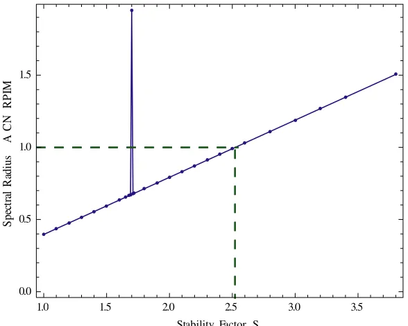
1.0 1.5 2.0 2.5 3.0 3.5

0.0 0.5 1.0 1.5

Stability Factor S

S

pect

ra

l

R

ad

iu

s

A

CN

R

P

IM

Figure 5. The spectral radius of the matrix A [CN-RPIM] versus stability factor S.

0.5% and 1.8% at the stability factors 1, 2 and 5, respectively. The accuracies of the simulated resonant frequencies, for the different stability factors, are very satisfactory. From these aforementioned numerical implementations we numerically deduce that the CN-RPIM is unconditionally stable.

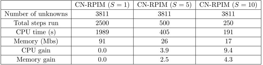
Table 1. Computational expenditure for 2-D rectangular ridged cavity.

CN-RPIM (S = 1) CN-RPIM (S= 5) CN-RPIM (S = 10)

Number of unknowns 3811 3811 3811

Total steps run 2500 500 250

CPU time (s) 1989 405 191

Memory (Mbs) 91 26 17

CPU gain 0.0 3.9 9.4

Memory gain 0.0 2.5 4.3

1.7, the spectral radius presents a singularity closely related to the characteristic stability limit of the RPIM, as mentioned in [13, 22] where its value is around S= 1.66.

The computational costs and memory requirements for the CN-RPIM are listed in Table 1, for the numerical computed structure. The CN-RPIM notably reduces the whole computational time as

S is increased. The unconditionally stable CN-RPIM reduces the CPU time by up to 90% when the stability factor is chosen to beS= 10, and the memory requirement is saved up to 81%. Therefore, the CN-RPIM reduces the computational expenditure with the increase of stability factor.

6. CONCLUSION

In this paper, the RPIM algorithm is implemented in conjunction with the Maxwell’s equations to solve electromagnetic problems in time-domain. To overcome the CFL limit on time-step, the CN scheme is implemented too in the previously mentioned algorithm to omit this condition on time-step. As a reminder, this time-step must comply with the Nyquist condition as an upper limit. Looking for the eigenvalues of the resulting linear system, the analytical calculus confirms that the spectral radius remains equal to unity independent of the prefixed RPIM spatial discretization and the time-step. We applied the CN-RPIM for a double-ridged cavity in order to have its first resonant frequency for different stability factors. We have numerically verified the agreement between the numerical obtained frequencies and those predicted by the theory. The unconditional stability of the CN-RPIM is justified analytically and confirmed numerically. In addition, the matrix inversion involved by the CN scheme is avoided and approximated if the stability factor S remains inferior to 2.525. The CN-RPIM permits a significant reduction of the computational expenditure; this is by increasing the stability factor. Although the CN-RPIM remains efficient, it reveals a little loss of accuracy.

APPENDIX A.

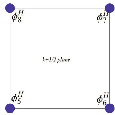
Here the Taflove and Umashankar notation is adopted for positioning the spread nodes [3]. Figure A1 reveals that any (ijk)E-node is surrounded by eight H-nodes, four H-nodes at the k −1/2 plane as presented by Figure A2 and four at the k+ 1/2 plane too, for Figure A3. The magnetic shape functions are arbitrarily indexed, and their derivatives are calculated at the considered (i, j, k)E-node. The presence of monomial terms in the interpolation Equation (1) improve the accuracy of the results and remove the impact of the shape parameter c on the H shape function derivatives evaluated at theE-node position [5] and vice versa. Obviously, the implementation of the RPIM algorithm for this uniform distribution gives numerically that:

∂φE_m ∂q =

∂φH_m ∂q =±

1

4.Δq for m∈[1,8] and q=x, y, z (A1)

Table A1. Sign of theH/E-shape function derivative versus the nodes location.

N ode1 N ode2 N ode3 N ode4 N ode5 N ode6 N ode7 N ode8

sign

∂φE,H

∂x

− + + − − + + −

sign

∂φE,H

∂y

− − + + − − + +

sign

∂φE,H

∂z

− − − − + + + +

Figure A1. Support domain of theE-node (i, j, k) and the neighboringH-nodes.

Figure A2. Projection of the E-node compact support on thek−1/2 plane.

Applying the discrete Fourier transform to Equation (22) outlines the field phasors function at the relative positions betweenH/E-nodes and the considered E/H-node; therefore, it follows:

εn_x,i+1X_iE=E_x,in X_iE+

Δt

2ε

1 4Δy

((−Exp [j(−k_xΔx−k_yΔy−k_zΔz) /2]Hn_z+1

−Exp [j(k_xΔx−k_yΔy−k_zΔz) /2]H_zn+1+ Exp [j(k_xΔx+k_yΔy−k_zΔz) /2]Hn_z+1 +Exp [j(−k_xΔx+k_yΔy−k_zΔz) /2]Hn_z+1−Exp [j(−k_xΔx−k_yΔy+k_zΔz) /2]H_zn+1

−Exp [j(+k_xΔx−k_yΔy+k_zΔz) /2]H_zn+1+ Exp [j(+k_xΔx+k_yΔy+k_zΔz) /2]Hn_z+1 +Exp [j(−k_xΔx+k_yΔy+k_zΔz) /2]Hn_z+1) + (−Exp [j(−k_xΔx−k_yΔy−k_zΔz) /2]Hn_z

−Exp [j(k_xΔx−k_yΔy−k_zΔz) /2]H_zn+ Exp [j(k_xΔx+k_yΔy−k_zΔz) /2]Hn_z +Exp [j(−k_xΔx+k_yΔy−k_zΔz) /2]Hn_z −Exp [j(−k_xΔx−k_yΔy+k_zΔz) /2]Hn_z

−Exp [j(+k_xΔx−k_yΔy+k_zΔz) /2]H_zn+ Exp [j(+k_xΔx+k_yΔy+k_zΔz) /2]Hn_z +Exp [j(−k_xΔx+k_yΔy+k_zΔz) /2]Hn_z))

−

Δt

2ε

1 4Δz

((−Exp [j(−k_xΔx−k_yΔy−k_zΔz) /2]Hn_y+1

−Exp [j(k_xΔx−k_yΔy−k_zΔz) /2]H_yn+1−Exp [j(+k_xΔx+k_yΔy−k_zΔz) /2]Hn_y+1

−Exp [j(−k_xΔx+k_yΔy−k_zΔz) /2]H_yn+1+ Exp [j(−k_xΔx−k_yΔy+k_zΔz) /2]H_yn+1 +Exp [j(+k_xΔx−k_yΔy+k_zΔz) /2]Hn_y+1+ Exp [j(+k_xΔx+k_yΔy+k_zΔz) /2]Hn_y+1 +Exp [j(−k_xΔx+k_yΔy+k_zΔz) /2]Hn_y+1) + (−Exp [j(−k_xΔx−k_yΔy−k_zΔz) /2]Hn_y

−Exp [j(k_xΔx−k_yΔy−k_zΔz) /2]H_yn−Exp [j(k_xΔx+k_yΔy−k_zΔz) /2]Hn_y

−Exp [j(−k_xΔx+k_yΔy−k_zΔz) /2]H_yn+ Exp [j(−k_xΔx−k_yΔy+k_zΔz) /2]Hn_y +Exp [j(+k_xΔx−k_yΔy+k_zΔz) /2]Hn_y + Exp [j(+k_xΔx+k_yΔy+k_zΔz) /2]Hn_y

+Exp [j(−k_xΔx+k_yΔy+k_zΔz) /2]Hn_y)), (A2) After some simplifications and adoptions of the transcendental notation, the right-hand side terms of Equation (A2) are generated:

εn_x,i+1X_iE = εn_x,iX_iE+

Δt

2ε

1

4Δy 8jCos

k_xΔx

2

Sin

k_yΔy

2

Cos

k_zΔz

2

Hn+1

z

+

8jCos

k_xΔx

2

Sin

k_yΔy

2

Cos

k_zΔz

2

Hn z

−

Δt

2ε

1

4Δz 8jCos

k_xΔx

2

Cos

k_yΔy

2

Sin

k_zΔz

2

Hn+1

y,j

+8jCos

k_xΔx

2

Cos

k_yΔy

2

Sin

k_zΔz

2

Hn_y,j

(A3)

Finally, Equation (38) is obtained, and similarly for the others.

εn_x+1 =εn_x +SyWy

ε H

n+1

z +Sy_εWyH n

z −

S_zW_z

ε H

n+1

y,j −

S_zW_z

ε H

n

y,j. (A4)

REFERENCES

1. Ramm, A. G., Inverse Problems Mathematical and Analytical Techniques with Applications to Engineering, Springer Science, 2005.

2. Collin, R. E.,Foundations of Microwave Engineering, IEEE Press Series on Electromagnetic Wave Theory, 2000.

4. Taflove, A. and S. C. Hagness, Computational Electrodynamics: The Finite Difference Time-Domain Method, Artech House, 2000.

5. Liu, G. R.,Mesh-Free Methods Moving beyond the Finite Element Method, CRC Press, 2003. 6. Ala, G., E. Francomano, A. Tortorici, E. Toscano, and F. Viola, “Smoothed particle

electromagnetics: A mesh-free solver for transients,” J. Comput. Appl. Math., Vol. 191, No. 2, 194–205, 2006.

7. Melenk, J. M. and I. Babuska, “The partition of unity finite element method: Basic theory and applications,” Comput. Meth. Appl. Mech. Eng., Vol. 139, 289–314, 1996.

8. Babuska, I. and J. M. Melenk, “The partition of unity method,” Int. J. Numer. Methods Eng., Vol. 40, 727–758, 1997.

9. Atluri, S. N., H. G. Kim, and J. Y. Cho, “A critical assessment of the truly meshless local Petrov-Galerkin (MLPG) and local boundary integral equation (LBIE) methods,” Comput. Mech., Vol. 24, No. 5, 348–372, November 1999.

10. Liu, G. R. and Y. T. Gu,An Introduction to Meshfree Methods and Their Programming, Springer, 2005.

11. Yu, Y., F. Jolani, and Z. Chen, “A hybrid ADI-RPIM scheme for efficient meshless modeling,” IEEE MTT-S Int. Microw. Symp. Dig., 1–4, 2011.

12. Zhu, H., C. Gao, and H. Chen, “An unconditionally stable radial point interpolation method based on Crank-Nicolson scheme,”IEEE Antennas and Wireless Propagation Letters, Vol. 16, 393, 2017. 13. Yu, Y. and Z. Chen, “Towards the development of an unconditionally stable time-domain meshless numerical method,” IEEE Transactions on Microwave Theory and Techniques, Vol. 58, No. 3, March 2010.

14. Hopfer, S., “The design of ridged waveguides,” IRE Transactions on Microwave Theory and Techniques, 20–29, October 1955.

15. Chen, T.-S., “Calculation of the parameters of the ridged waveguides,” IRE Transactions on Microwave Theory and Techniques, 12–17, January 1957.

16. Rong, Y. and K. A. Zak, “Characteristics of generalized rectangular and circular ridge waveguides,” IEEE Transactions on Microwave Theory and Techniques, Vol. 48, No. 2, 258–265, 2000.

17. Kim, H., I.-S. Koh, and J.-G. Yook, “Implicit ID-FDTD algorithm based on Crank-Nicolson scheme: Dispersion relation and stability analysis,” IEEE Transactions on Antennas and Propagation, Vol. 59, No. 6, June 2011.

18. Meurant, G.,Computer Solution of Large Linear Systems, Elsevier, 2006.

19. Balanis, C. A.,Advanced Engineering Electromagnetics, John Wiley and Sons, 1989. 20. Marcuvirz, N.,Waveguide Handbook, Peter Peregrinus Ltd., 1965.

21. Sun, G. and C. W. Trueman, “Efficient implementations of the Crank-Nicolson scheme for the finite-difference time-domain method,” IEEE Transactions on Microwave Theory and Techniques, Vol. 54, No. 5, May 2006.