Volume 2006, Article ID 59587, Pages1–6 DOI 10.1155/ASP/2006/59587
Generalized Sampling Theorem for Bandpass Signals
Ales Prokes
Department of Radio Electronics, Brno University of Technology, Purkynova 118, 612 00 Brno, Czech Republic
Received 29 September 2005; Revised 19 January 2006; Accepted 26 February 2006
Recommended for Publication by Yuan-Pei Lin
The reconstruction of an unknown continuously defined function f(t) from the samples of the responses ofmlinear time-invariant (LTI) systems sampled by the 1/mth Nyquist rate is the aim of the generalized sampling. Papoulis (1977) provided an elegant solution for the case where f(t) is a band-limited function with finite energy and the sampling rate is equal to 2/m times cutofffrequency. In this paper, the scope of the Papoulis theory is extended to the case of bandpass signals. In the first part, a generalized sampling theorem (GST) for bandpass signals is presented. The second part deals with utilizing this theorem for signal recovery from nonuniform samples, and an efficient way of computing images of reconstructing functions for signal recovery is discussed.
Copyright © 2006 Hindawi Publishing Corporation. All rights reserved.
1. INTRODUCTION
A multichannel sampling involves passing the signal through distinct transformations before sampling. Typical cases of these transformations treated in many works are delays [2– 6] or differentiations of various orders [7]. A generalization of both these cases on the assumption that the signal is repre-sented by a band-limited time-continuous real function f(t) with finite energy was introduced in [1] and developed in [8].
Under certain restrictions mentioned below, a similar generalization can be formed for bandpass signals repre-sented by a function f(t) whose spectrumF(ω) is assumed to be zero outside the bands (−ωU,−ωL) and (ωL,ωU) as
de-picted inFigure 1(a)while its other properties are identical as in the case of bandpass signals.
If a signal is undersampled (i.e., a higher sampling order is used), then its original spectrum components and their replicas overlap and the frequency intervals (ωL,ωU) and
(−ωU,ωL) are divided into several subbands, whose number
depends for given frequenciesωU andωLon the sampling
frequencyωS, [4,9].
For the introduction of GST, the number of overlapped spectrum replicas has to agree with the sampling orderm, with the number of subbands inside the frequency ranges (ωL,ωU) and (−ωU,−ωL), and with the number of linear
systems. As presented in [9], to meet the above demands, m must be an even number and the sampling frequency ωS=2π/TS, whereTSis the sampling period, and bandwidth
ωB=ωU−ωLhas to meet the following conditions:
ωL
ωU−ωL =
ωL
ωB =
k0
m, (1)
wherek0is any positive integer number, and
ωS
ωB =
2
m. (2)
An example of a fourth-order sampled signal spectrum in the vicinity of positive and negative original spectral com-ponents, if conditions (1) and (2) are fulfilled, is shown in Figure 1(b)andFigure 1(c).
Figure 2shows a graphical interpretation of the sampling ordersm=2 to 6 in the planeωS/ωB versusωC/ωB, where
ωC =(ωU +ωL)/2, if the common case of bandpass signal
sampling is assumed (i.e., frequencyωSfor givenωBandωC
is chosen arbitrary) [4,9]. Odd orders correspond to the grey areas, whereas even orders correspond to the white ones. The solutions of (1) and (2) fork0 =0, 1, 2,. . .whenm=2 and
m=4 are marked by black points.
2. GENERALIZED SAMPLING THEOREM FOR
BANDPASS SIGNALS
F(ω)
−ωU−ωC−ωL ωL ωC ωU ω
(a)
Gsi(ω)
ωL−ωC+ (k0+ 1)ωS ωU ω (b)
Gs i(ω)
−ωU ωC−(k0+ 1)ωS −ωL ω (c)
Figure1: (a) Spectrum of bandpass signal, spectrum of sampled responsesgi(t) at the output of LTI prefilters in the vicinity of (b)
positive and (c) negative original spectrum components.
system functions
H1(ω),H2(ω),. . .,Hm(ω). (3)
The output functions of all prefilters
gi(t)= 1
2π −ωL
−ωU
F(ω)Hi(ω)ejωtdω
+ 1 2π
ωU
ωL
F(ω)Hi(ω)ejωtdω
(4)
are then sampled at 1/mth Nyquist rate related to the cut-offfrequency ωB. If mutual independence of the prefilters
is assumed and if no noise is present in the system, func-tion f(t) can be exactly reconstructed from samplesgi(nTS),
whereTS=mπ/ωB.
For this purpose, the following system of equations has to be formed:
HY=R, (5)
where matrix H and vectorsY andR are of the following form: H= ⎡ ⎢ ⎢ ⎢ ⎢ ⎢ ⎢ ⎢ ⎢ ⎢ ⎢ ⎢ ⎢ ⎢ ⎢ ⎢ ⎢ ⎢ ⎢ ⎢ ⎢ ⎢ ⎢ ⎢ ⎢ ⎢ ⎢ ⎢ ⎣
H1(ω), H2(ω), · · · Hm(ω)
H1
ω+ωS
, H2
ω+ωS
, · · · Hm
ω+ωS
.. . ... ... H1 ω+ m
2 −1 ωS , H2
ω+
m
2 −1 ωS , · · · Hm
ω+
m 2 −1 ωS
H1
ω+
m
2 +k0 ωS , H2
ω+
m
2 +k0 ωS , · · · Hm
ω+
m
2 +k0 ωS
H1
ω+
m
2 +k0+ 1 ωS , H2
ω+
m
2 +k0+ 1 ωS , · · · Hm
ω+
m
2 +k0+ 1 ωS ..
. ... ...
H1
ω+k0+m−1
ωS
, H2
ω+k0+m−1
ωS
, · · · Hm
ω+k0+m−1
ωS ⎤ ⎥ ⎥ ⎥ ⎥ ⎥ ⎥ ⎥ ⎥ ⎥ ⎥ ⎥ ⎥ ⎥ ⎥ ⎥ ⎥ ⎥ ⎥ ⎥ ⎥ ⎥ ⎥ ⎥ ⎥ ⎥ ⎥ ⎥ ⎦ , (6) Y= ⎡ ⎢ ⎢ ⎢ ⎢ ⎢ ⎢ ⎢ ⎢ ⎢ ⎢ ⎢ ⎢ ⎢ ⎢ ⎢ ⎢ ⎢ ⎢ ⎢ ⎣
Y1(ω,t)
Y2(ω,t) · · · · · · · · · · · ·
Ym−1(ω,t)
Ym(ω,t)
⎤ ⎥ ⎥ ⎥ ⎥ ⎥ ⎥ ⎥ ⎥ ⎥ ⎥ ⎥ ⎥ ⎥ ⎥ ⎥ ⎥ ⎥ ⎥ ⎥ ⎦
, R= ⎡ ⎢ ⎢ ⎢ ⎢ ⎢ ⎢ ⎢ ⎢ ⎢ ⎢ ⎢ ⎢ ⎢ ⎢ ⎢ ⎢ ⎢ ⎢ ⎢ ⎢ ⎢ ⎢ ⎢ ⎢ ⎢ ⎢ ⎣ 1
expjωSt
.. . exp j m
2 −1 ωSt
exp
j
m
2 +k0 ωSt
exp
j m
2 +k0+ 1 ωSt ..
.
expjk0+m−1
ωSt
0.4 0.5 0.6 0.7 0.8 0.9 1 1.1
ωS
/ω
B
0.5 1 1.5 2 2.5 3 3.5 4
ωC/ωB
k0=0 k0=1 k0=2
k0=0 k0=2 k0=4
m=2
m=3
m=4
m=5
m=6
Figure2: Graphical interpretation of the sampling orders.
In the above formulaetis any number andω∈(−ωU,−ωU+
ωS). This system definesmfunctions
Yi(ω,t),Y2(ω,t),. . .,Ym(ω,t) (8)
ofωandtbecause the coefficients in matrixHdepend onω and the right-hand side depends ont.FunctionsHi(ω) are
on the one hand general, but on the other hand they cannot be entirely arbitrary: they must meet the condition that the determinant of the matrix of coefficients differs from zero for everyω∈(−ωU,−ωU+ωS).
Since the sampled responsesgis(t) are of the form
gs
i(t)=gi(t) ∞
n=−∞
δt−nTs
, i=1, 2,. . .,m, (9)
the function f(t) at the output of the multichannel sampling configuration can be described by the following formula:
f(t)= m
i=1
gs
i(t)∗yi(t)= m
i=1
∞
n=−∞
gi
nTs
yi
t−nTs
,
(10)
where
yi(t)= Ts
2π
−ωU+ωS
−ωU
Yi(ω,t)ejωtdω, i=1,. . .,m. (11)
The GST ((5), (10), and (11)) can be proven in a similar way as published in [1].
If we assume thatk0 = 0 and put it into (1), then we
obtainωL = 0. It means that the bandpass function turns
into the band-limited function with cutofffrequencyωBand
the above sampling theorem turns into a generalized sam-pling expansion [1]. We can say that [1] is a special case of the above GST.
H1(ω)
H2(ω)
Hm(ω)
Y1(ω,t)
Y2(ω,t)
Ym(ω,t)
f(t) f(t)
g1(t)
g2(t)
gm(t)
gs1(t)
gs2(t)
gs m(t)
f1(t)
f2(t)
fm(t) +
×
×
×
. . .
. . .
nδ
t−nTs
Figure3: Multichannel sampling configuration.
3. FUNCTION RECOVERY FROM NONUNIFORM
SPACED SAMPLES
As one of the typical applications of the GST, the reconstruc-tion of a signal f(t) from periodically repeated groups of nonuniform spaced samples can be considered [2–5]. It can be obtained if the following formulae hold:
Hi(ω)=ejαiω,
Hi
ω+qωs
=Hi(ω)ejαiqωs,
(12)
whereαidenotes time delay inith branch, that is, the distance
betweenith sample and the centre of the group.
Substituting (12) into (6), a set of linear equations is ob-tained, which can be solved by Cramer’s rule [10]. For this purpose, (m+ 1) determinants of the following types have to be solved:
D= m
i=1
Hi(ω)
1 1 . . . 1
s1, s2, . . . sm
s21, s22, . . . s2m
..
. ... ... ...
s1m/2−1, s2m/2−1, . . . sm/m2−1
s(m/2+k0) 1 , s
(m/2+k0)
2 , . . . s (m/2+k0)
m
s(m/2+k0+1) 1 , s(
m/2+k0+1) 2 , . . . s(
m/2+k0+1)
m
..
. ... ... ...
s(m/2+k0−1) 1 , s
(m/2+k0−1) 2 , . . . s
(m/2+k0−1)
m
,
(13)
wheresi=ejαiωs,i=1, 2,. . .,m. Then (11) and consequently
lower part of determinant. Finding systematic results, which can be explored for reconstruction, is problematic. A possi-bly way for m > 2 andk0 ≥ 1 consists in transformation
of (13) into Vandermonde’s form by appending the auxiliary termsX1,X2,X3, andS2:
DV = m
i=1
Hi(ω)
X1, S1
X2, S2
X3, S3
= m i=1
Hi(ω), (14)
where =
1, . . . 1, 1, . . . 1
x1, . . . xk0, S1, . . . Sm ..
. ... ... ... ... ...
x(1m/2−1), . . . x (m/2−1)
k0 , S
(m/2−1)
1 , . . . S (m/2−1)
m
x1(m/2), . . . x(km/0 2), S (m/2)
1 , . . . S(mm/2)
..
. ... ... ... ... ...
x(m/2+k0−1) 1 , . . . x(
m/2+k0−1)
k0 , S
(m/2+k0−1) 1 , . . . S(
m/2+k0−1)
m
x(m/2+k0)
1 , . . . x (m/2+k0)
k0 , S
(m/2+k0)
1 , . . . S (m/2+k0)
m
x(m/2+k0+1) 1 , . . . x(
m/2+k0+1)
k0 , S
(m/2+k0+1) 1 , . . . S(
m/2+k0+1)
m
..
. ... ... ... ... ...
x(m+k0−1)
1 , . . . x (m+k0−1)
k0 , S
(m+k0−1)
1 , . . . S (m+k0−1)
m (15)
and in using of Vandermonde’s rule
DV= m
i=1
Hi(ω)· m−1
i=1
m
j=i+1
sj−si
· k0 i=1 m j=1 sj−xi
· k0−1
i=1
k0
j=i+1
xj−xi
.
(16)
The intermediate term can be rewritten in the following form: k0 i=1 m j=1 sj−xi
=
s1−x1 s2−x1
· · · sm−x1
·s1−x2 s2−x2
· · · sm−x2
.. .
·s1−xk0 s2−xk0
· · · sm−xk0
=
xm
1 −σ1xm−1 1+σ2xm−1 2− · · ·+ (−1)mσm
·xm
2 −σ1xm−2 1+σ2x2m−2− · · ·+ (−1)mσm
.. .
·xkm0−σ1x
m−1
k0 +σ2x
m−2
k0 − · · ·+ (−1)
mσ m
, (17)
whereσkare symmetric polynomials consisting of products
of all the permutations ofk=1, 2,. . .,mtermss1,s2,. . .,sm.
That is,
σ1=s1+s2+· · ·+sm,
σ2=s1s2+s1s3+· · ·+s1sm
+s2s3+· · ·+s2sm+· · ·+sm−1sm,
.. .
σm=s1s2· · ·sm.
(18)
Finally, we assume that determinant Δ in (14) is ex-panded according to the intermediate band ofX2,S2 using
the Laplace expansion. Because the desired determinant (13) (termsS1andS3) is an algebraic complement of termX2, it
can be revealed as a factor in every multiplication of all the permutations ofk0terms of block X2in the result of (17).
Therefore, only one product corresponding to the main di-agonal or an adjacent one of the subdeterminantX2is suffi
-cient. For the final expression of result, special cases of sym-metric polynomials have to be defined. They areσ0=1 and
σk=0 fork <0 andk > m.
In this way, determinant (13) is obtained in the form
D= m
i=1
Hi(ω)· m−1
i=1
m
j=i+1
sj−si
·(−1)k0(k0−1)/2
σm/2−k0+1, σm/2−k0+2, · · · σm/2 σm/2−k0+2, σm/2−k0+3, · · · σm/2+1
..
. ... ... ... σm/2, σm/2+1, · · · σm/2+k0−1
. (19)
In a similar way, the determinantsDi,i = 1, 2,. . .,m,
which can be formed by replacing the ith column vector with the right-hand side vectorR, can be computed. Finally, the desired functionsYi(ω,t) can be obtained from the ratio
Di/D.
The determinant in (19) is called the per-symmetric de-terminant. In the casek0≥m, it contains nonzero terms only
near the secondary diagonal.
The efficiency of the described method depends on the values k0 andm. It is very high in the case k0 < m,
be-cause the order of the determinant that has to be computed is lower than the order of determinant (13), and the result-ing expression of (19) contains a large amount of products (sj−si), some of which vanish due to divisionsDi/D.
Func-tionsYi(ω,t) are then obtained in a very simple form. Ifk0
increases, the determinant order in (19) also increases while the efficiency decreases. In the casek0 >> m, the order
ap-proaches the value 2k0. Although the determinant contains
4. EXAMPLE OF GST APPLICATION
Although a band-limited function with finite energy is as-sumed in paragraph 1, in reality most the signals can be re-garded as time-unlimited. A simple example (m=2) of a sig-nal with infinite-energy recovery is shown below. By choos-ingH1(ω)=1 andH2(ω)=ejαωand substituting them into
(10), we obtain
1, ejαω
1, ejα[ω+(k0+1)ωs]
·
Y1(ω,t)
Y2(ω,t)
=
1 ejα(k0+1)ωst
. (20)
The images of reconstructing functionsY1(ω,t) andY2(ω,t)
can be found in the form
Y1(ω,t)=ej((k0+1)/2)ωst
sink0+ 1
/2ωs(t−α)
sink0+ 1
ωsα/2
,
Y2(ω,t)=ej((k0+1)/2)ωst(t−α)ejωα
sink0+ 1
ωst/2
sink0+ 1
ωsα/2
.
(21)
By evaluating (11) under the condition that ωS = ωB, the
reconstructing functions can be expressed as
y1(t)= −sinc
πt Ts
sink0+ 1
πt−α/Ts
sink0+ 1
πα/Ts
,
y2(t)=sinc
π(t−α) Ts
sink0+ 1
πt/Ts
sink0+ 1
πα/Ts
,
(22)
where sinc(x)=sin(x)/x. The final reconstruction (10) from a limited number of sample groupsncan be rewritten in the form
fr(t)= f
nTs
y1
t−nTs
+ fnTs+α
y2
t−nTs
. (23)
In accordance with (1) and (2), the bandwidth, sampling fre-quency, carrier frefre-quency, and coefficient k0 are chosen as
follows:ωB=π/2 rad/s,ωS=π/2 rad/s,ωC=2πrad/s, and
k0=7.
Let function f(t) be given by the formula f(t) = [1 + 0.5(sinω1t+ sinω2t)] cos 2πt. The spectrum of f(t) is then
composed of five Dirac pulses at the frequencies 2π±ω1, 2π±
ω2, and 2π. To demonstrate the reconstruction of a function
whose spectrum is inside or partially outside the frequency interval (ωL,ωU), the modulation frequencies of f(t) were
chosen as follows:ω1 =0.2 rad/s,ω2 =0.6 rad/s, andω2 =
0.85 rad/s.
Reconstructing functions y1(t) and y2(t) are shown in
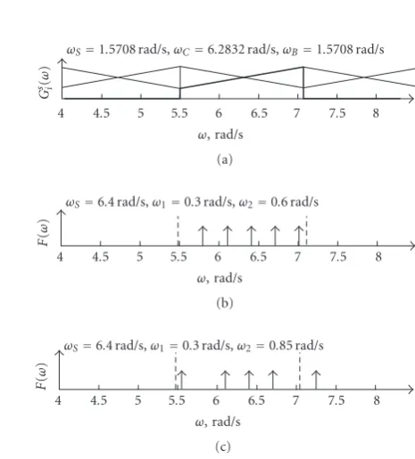
Figure 4. The relation between spectrumF(ω) and the spec-trum of sampled common responsesGsi(ω) is shown in
Fig-ure 5.
−10 −5 0 5 10
t,s
−1 0 1
y1(t)
y2(t)
α=0.25 s
Figure4: Reconstructing functionsy1(t) andy2(t).
G
s i(ω
)
4 4.5 5 5.5 6 6.5 7 7.5 8
ω, rad/s
ωS=1.5708 rad/s,ωC=6.2832 rad/s,ωB=1.5708 rad/s
(a)
F
(
ω
)
4 4.5 5 5.5 6 6.5 7 7.5 8
ω, rad/s
ωS=6.4 rad/s,ω1=0.3 rad/s,ω2=0.6 rad/s
(b)
F
(
ω
)
4 4.5 5 5.5 6 6.5 7 7.5 8
ω, rad/s
ωS=6.4 rad/s,ω1=0.3 rad/s,ω2=0.85 rad/s
(c)
Figure5: (a) Spectrum of sampled responses in the vicinity of pos-itive original spectrum component form=2. Spectrum of f(t) for both cases of modulation frequenciesω1andω2(b), (c).
Function f(t) and its reconstruction fr(t) from seven
groups of samplesn ∈ [−3, 3] are plotted inFigure 6. It is obvious that in the case of an aliasing occurrenceFigure 6(b), the reconstruction exhibits a measurable error.
5. CONCLUSION
A generalized sampling theorem for time-continuous band-pass signal and the application of this theorem to signal re-covery from nonuniform samples have been presented. An efficient method of computing the Fourier images of recon-structing functions for signal recovery from periodically re-peated groups of nonuniform spaced samples has then been discussed. As mentioned above, the method presented is suit-able for lower values ofk0(wideband applications). Finding
a simplification similar to (19) in the casek0>> m
−1 0 1
−16 −12 −8 −4 0 4 8 12 16
t,s
ωS=6.4 rad/s,ω1=0.3 rad/s,ω2=0.6 rad/s,
f(t)
fr(t)
Samples
(a)
−1 0 1
−16 −12 −8 −4 0 4 8 12 16
t,s
ωS=6.4 rad/s,ω1=0.3 rad/s,ω2=0.85 rad/s,
f(t)
fr(t)
(b)
Figure6: Function f(t) and its reconstruction fr(t) in cases that
spectrum of f(t) is (a) inside or (b) outside frequency interval (ωL,ωU). (TS=4 s,n∈[−3, 3],α=0.25 s.)
Note that in the case of frequency-limited signal recov-ery (k0=0), the determinant of symmetrical polynomials is
equal to one and the solution is very simple.
ACKNOWLEDGMENT
This work has been supported by the Grant GACR (Czech Science Foundation) no. 102/04/0557 “Development of the Digital Wireless Communication Resources,” and by the Re-search Programme MSM0021630513 “Advanced Electronic Communication Systems and Technologies.”
REFERENCES
[1] A. Papoulis, “Generalized sampling expansion,”IEEE Trans-actions on Circuits and Systems, vol. 24, no. 11, pp. 652–654, 1977.
[2] A. Kohlenberg, “Exact interpolation of band-limited func-tions,”Journal of Applied Physics, vol. 24, no. 12, pp. 1432– 1436, 1953.
[3] D. A. Linden, “A discussion of sampling theorems,” Proceed-ings of the IRE, vol. 47, pp. 1219–1226, 1959.
[4] A. J. Coulson, “A generalization of nonuniform bandpass sam-pling,”IEEE Transactions on Signal Processing, vol. 43, no. 3, pp. 694–704, 1995.
[5] Y.-P. Lin and P. P. Vaidyanathan, “Periodically nonuniform sampling of bandpass signals,”IEEE Transactions on Circuits and Systems II: Analog and Digital Signal Processing, vol. 45, no. 3, pp. 340–351, 1998.
[6] Y. C. Eldar and A. V. Oppenheim, “Filterbank reconstruction of bandlimited signals from nonuniform and generalized sam-ples,”IEEE Transactions on Signal Processing, vol. 48, no. 10, pp. 2864–2875, 2000.
[7] D. A. Linden and N. M. Abramson, “A generalization of the sampling theorem,”Information and Control, vol. 3, no. 1, pp. 26–31, 1960.
[8] J. Brown Jr., “Multi-channel sampling of low-pass signals,” IEEE Transactions on Circuits and Systems, vol. 28, no. 2, pp. 101–106, 1981.
[9] A. Prokeˇs, “Parameters determining character of signal spec-trum by higher order sampling,” inProceedings of the 8th In-ternational Czech-Slovak Scientific Conference (Radioelektron-ika ’98), vol. 2, pp. 376–379, Brno, Czech Republic, June 1998. [10] C. D. Meyer, Matrix Analysis and Applied Linear Algebra,
SIAM, Philadelphia, Pa, USA, 2000.
Ales Prokeswas born in Znojmo, Czech Re-public, in 1963. He received the M.S. and Ph.D. degrees in electrical engineering from the Brno University of Technology, Czech Republic, in 1988 and 2000, respectively. He is currently an Assistant Professor at the Brno University of Technology, Depart-ment of Radio Electronics. His research in-terests include nonuniform sampling, ve-locity measurement based on spatial