Novel VLSI Algorithm and Architecture with Good Quantization Properties for a High-Throughput Area Efficient Systolic Array Implementation of DCT

(1)

Volume 2011, Article ID 639043,14pages doi:10.1155/2011/639043

Research Article

Novel VLSI Algorithm and Architecture with Good

Quantization Properties for a High-Throughput Area

Efficient Systolic Array Implementation of DCT

Doru Florin Chiper and Paul Ungureanu

Faculty of Electronics, Telecommunications and Information Technology, Technical University “Gh. Asachi”, B-dul Carol I, No.11, 6600 Iasi, Romania

Correspondence should be addressed to Doru Florin Chiper,[email protected]

Received 31 May 2010; Revised 18 October 2010; Accepted 22 December 2010

Academic Editor: Juan A. L ´opez

Copyright © 2011 D. F. Chiper and P. Ungureanu. This is an open access article distributed under the Creative Commons Attribution License, which permits unrestricted use, distribution, and reproduction in any medium, provided the original work is properly cited.

Using a specific input-restructuring sequence, a new VLSI algorithm and architecture have been derived for a high throughput memory-based systolic array VLSI implementation of a discrete cosine transform. The proposed restructuring technique transforms the DCT algorithm into a cycle-convolution and a pseudo-cycle convolution structure as basic computational forms. The proposed solution has been specially designed to have good fixed-point error performances that have been exploited to further reduce the hardware complexity and power consumption. It leads to a ROM based VLSI kernel with good quantization properties. A parallel VLSI algorithm and architecture with a good fixed point implementation appropriate for a memory-based implementation have been obtained. The proposed algorithm can be mapped onto two linear systolic arrays with similar length and form. They can be further eﬃciently merged into a single array using an appropriate hardware sharing technique. A highly eﬃcient VLSI chip can be thus obtained with appealing features as good architectural topology, processing speed, hardware complexity and I/O costs. Moreover, the proposed solution substantially reduces the hardware overhead involved by the pre-processing stage that for short length DCT consumes an important percentage of the chip area.

1. Introduction

The discrete cosine transform (DCT) and discrete sine transform (DST) [1–3] are key elements in many digital signal processing applications being good approximations to the statistically optimal Karhunen-Loeve transform [2,3]. They are used especially in speech and image transform coding [3,4], DCT-based subband decomposition in speech and image compression [5], or video transcoding [6]. Other important applications are: block filtering, feature extraction [7], digital signal interpolation [8], image resizing [9], transform-adaptive filtering [10, 11], and filter banks [12].

The choice of DCT or DST depends on the statistical properties of the input signal. For low correlated input

signals, DST oﬀers a lower bit rate [3]. For high correlated input signals, DCT is a better choice.

Prime-length DCTs are critical for a prime-factor algo-rithm (PFA) technique to implement DCT or DST. PFA technique can be used to significantly reduce the overall complexity [13] that results in higher-speed processing and reduced hardware complexity. PFA can split aN =N1×N2

point DCT, where N1 and N2 are mutually primes, into a two-dimensionalN1×N2DCT. DCT is then applied for each

dimension, and the results are combined through input and output permutations.

(2)

although many eﬀorts have been made to reduce the computational complexity [14, 15]. Thus, it is necessary to reformulate or to find new VLSI algorithms for these transforms. These hardware algorithms have to be designed appropriately to meet the system requirements. To meet the speed and power requirements, it is necessary to appropri-ately exploit the concurrency involved in such algorithms. Moreover, the VLSI algorithm and architecture have to be derived in a synergetic manner [16].

The data movement into the VLSI algorithm plays an important role in determining the eﬃciency of a hardware algorithm. It is well known that FFT, which plays in important role in the software implementation of DFT, is not well suited for VLSI implementation. This is one explanation why regular computational structures such as cyclic convolution and circular correlation have been used to obtain eﬃcient VLSI implementations [17–19] using modular and regular architectural paradigm as distributed arithmetic [20] or systolic arrays [21]. This approach leads to low I/O cost and reduced hardware complexity, high speed and a regular and modular hardware structure.

Systolic arrays are an appropriate architectural paradigm that leads to eﬃcient VLSI implementations that meet the increased speed requirements of real-time applications through an eﬃcient exploitation of concurrency involved in the algorithms. This paradigm is well suited to the character-istics of the VLSI technology through its modular and regular structure with local and regular interconnections.

Owing to regular and modular structure of ROMs, memory-based techniques are more and more used in the recent years. They offer also a low hardware complexity and high speed for relatively small sizes compared with the multiplier-based architectures. Multipliers in such archi-tectures [22–25] consume a lot of silicon area, and the advantages of the systolic array paradigm are not evident for such architectures. Thus, memory-based techniques lead to cost-effective and efficient VLSI implementations.

One memory-based technique is the distributed arith-metic (DA). This technique is largely used in commercial products due to its eﬃcient computation of an inner-product. It is faster then multiplier-based architecture due to the fact that it uses precomputed partial results [26,27]. However, the ROM size increases exponentially with the transform length, even if a lot of work have been done to reduce its complexity as in [28], rendering this technique impractical for large sizes. Moreover, this structure is diﬃcult to pipeline.

The other main technique is the direct-ROM implemen-tation of multipliers. In this case, multipliers are replaced with ROlM-based look-up table (LUT) of size 2LwhereLis the word length. The 2Lpre-computed values of the product for all possible values of the input are stored in the ROM.

In [16, 19], another memory-based technique that combines the advantages of the systolic arrays with those of memory-based designs is used. This technique will be called memory-based systolic arrays. When the systolic array paradigm is used as a design instrument, the advantages are evident only when a large number of processing elements can be integrated on the same chip. Thus, it is very important to

reduce the PE chip area using small ROMs as it is proposed in this technique.

In this paper, a new parallel VLSI algorithm for a prime-length Discrete Cosine Transform (DCT) is proposed. It significantly simplifies the conversion of the DCT algorithm into a cycle and a pseudo-cycle convolution using only a new single input restructuring sequence. It can be used to obtain an efficient VLSI architecture using a linear memory-based systolic array. The proposed algorithm and its associated VLSI architecture have good numerical properties that can be efficiently exploited to lead to a low-complexity hardware implementation with low power consumption. It uses a cycle and a pseudo-cycle convolution structure that can be efficiently mapped on two linear systolic arrays having the same form and length and using a small number of I/O channels placed at the two extreme ends of the array. The proposed systolic algorithm uses an appropriate parallelization method that efficiently decomposes DCT into a cycle and a pseudo-cycle convolution structure, obtaining thus a high throughput. It can be efficiently computed using two linear systolic arrays and an appropriate control structure based on the tag-control scheme. The proposed approach is based on an efficient parallelization scheme and an appropriate reordering of these sequences using the properties of the Galois Field of the indexes and the symmetry property of the cosine transform kernel. Thus, using the proposed algorithm, it is possible to obtain a VLSI architecture with advantages similar to those of systolic array and memory-based implementations using the benefit of the cycle convolution. Thus a high speed, low I/O cost, and reduced hardware complexity with a high regularity and modularity can be obtained. Moreover, the hardware overhead involved by the preprocessing stage can be substantially reduced as compared to the solution proposed in [16].

The paper is organized as follows. In Section 2, the new computing algorithm for DCT encapsulated into the memory-based systolic array is presented. InSection 3, two examples for the particular lengths N = 7 and N = 11 are used to illustrate the proposed algorithm. InSection 4, aspects of the VLSI design using the memory-based systolic array paradigm and a discussion on the eﬀects of a finite precision implementation are presented. In Section 5, the quantization properties of the proposed algorithm and architecture are analyzed analytically and by computer simulation. In Section 6, comparisons with similar VLSI designs are presented together with a brief discussion on the eﬃciency of the proposed solution. Section 7contains the conclusions.

2. Systolic Algorithm for 1D DCT

For the real input sequencex(i) :i=0, 1,. . .,N−1, 1D DCT is defined as

X(k)=

2 N ·

N−1

i=0

(3)

fork=1,. . .,N

withα= π

2N. (2)

To simplify the presentation, the constant coeﬃcient√2/N will be dropped from (1) that represents the definition of DCT; a multiplier will be added at the end of the VLSI array to scale the output sequence with this constant.

We will reformulate relation (1) as a parallel decomposi-tion based on a cycle and a pseudo-cycle convoludecomposi-tion forms using a single new input restructuring sequence as opposed to [16] where two such auxiliary input sequences were used. Further, we will use the proprieties of DCT kernel and those of the Galois Field of indexes to appropriately permute the auxiliary input and output sequences.

Thus, we will introduce an auxiliary input sequence {xa(i) : i = 0, 1,. . .,N−1}. It can be recursively defined as follows:

xa(N−1)=x(N−1), (3)

xa(i)=(−1)ix(i) +xa(i+ 1), (4)

fori=N−2,. . ., 0.

Using this restructuring input sequence, we can reformu-late (1) as follows:

X(0)=xa(0) + 2 N−1

i=0

(−1)ϕ(i)

×

xaϕ(i)−xa

ϕi+(N−1)

2 ,

X(k)=[xa(0) +T(k)]·cos(kα), fork=1,. . .,N−1.

(5)

The new auxiliary output sequence{T(k) : k = 1, 2, . . .,N−1}can be computed in parallel as a cycle and pseudo-cycle convolutions if the transform length N is a prime number as follows:

T(δ(k))=

(N−1)/2

i=1

(−1)ξ(k,i)

·

xaϕ(i−k)−xa

ϕi−k+(N−1) 2

×2·cosψ(i)×2α,

Tγ(k)=

(N−1)/2

i=1

(−1)ζ(i)

·

xaϕ(i−k)+xa

ϕi−k+(N−1) 2

×2·cosψ(i)×2α fork=0, 1,. . .,(N−1)

2 ,

(6)

where

ψ(k)= ⎧ ⎪ ⎨ ⎪ ⎩

ϕ₍_k₎ _if_ϕ₍_k₎_≤(N−1)

2 ,

ϕ₍_N₋_{1 +}_k₎ _otherwise, (7)

with

ϕ₍_k₎₌ ⎧ ⎨ ⎩

ϕ(k) ifk >0, ϕ(N−1 +k) otherwise

ϕ(k)=gk_N_,

, (8)

wherexN denotes the result ofx moduloN andg is the

primitive root of indexes.

We have also used the properties of the Galois Field of indexes to convert the computation of DCT as a convolution form.

3. Examples

To illustrate our approach, we will consider two examples for 1D DCT, one with the lengthN =7 and the primitive root g=3 and the other with the lengthN=11 and the primitive rootg=2.

3.1. DCT Algorithm with Length N = 7. We recursively compute the following input auxiliary sequence{xa(i) : i= 0,. . .,N−1}as follows:

xa(6)=x(6),

xa(i)=(−1)ix(i) +xa(i+ 1), fori=5,. . ., 0.

(9)

Using the auxiliary input sequence{xa(i) :i=0,. . .,N−1},

we can write (6) in a matrix-vector product form as

⎡ ⎢ ⎢ ⎢ ⎣

T(4) T(2) T(6) ⎤ ⎥ ⎥ ⎥ ⎦

= ⎡ ⎢ ⎢ ⎢ ⎣

−[xa(3)−xa(4)] −[xa(2)−xa(5)] −[xa(6)−xa(1)] [xa(6)−xa(1)] xa(3)−xa(4) −[xa(2)−xa(5)]

xa(2)−xa(5) −[xa(6)−xa(1)] xa(3)−xa(4)

⎤ ⎥ ⎥ ⎥ ⎦

· ⎡ ⎢ ⎢ ⎢ ⎣

c(2) c(1) c(3) ⎤ ⎥ ⎥ ⎥ ⎦,

(4)

⎡ ⎢ ⎢ ⎢ ⎣ T(3) T(5) T(1) ⎤ ⎥ ⎥ ⎥ ⎦ = ⎡ ⎢ ⎢ ⎢ ⎣

xa(3) +xa(4) xa(2) +xa(5) xa(6) +xa(1)

xa(6) +xa(1) xa(3) +xa(4) xa(2) +xa(5)

xa(2) +xa(5) xa(6) +xa(1) xa(3) +xa(4)

⎤ ⎥ ⎥ ⎥ ⎦ · ⎡ ⎢ ⎢ ⎢ ⎣ c(2) −c(1) −c(3) ⎤ ⎥ ⎥ ⎥ ⎦, (11)

where we have notedc(k) for 2·cos(2kα).

The index mappingsδ(i) andγ(i) realize a partition into two groups of the permutation of indexes {1, 2, 3, 4, 5, 6}. They are defined as follows:

{δ(i) : 1−→4, 2−→2, 3−→6},

γ(i) : 1−→3, 2−→5, 3−→1. (12)

The functionsξ(k,i) andζ(i) define the sign of terms in (10), respectively, as follows:

ξ(k,i) is defined by the matrix

1 1 1 0 0 1 0 1 0 and ζ(i) is defined by the vector [0 1 1].

Finally, the output sequence{X(k) :k=1, 2,. . .,N−1}can be computed as

X(1)=[xa(0) +T(1)]·cos[α],

X(2)=[xa(0) +T(2)]·cos[2α],

X(3)=[xa(0) +T(3)]·cos[3α],

X(4)=[xa(0) +T(4)]·cos[4α],

X(5)=[xa(0) +T(5)]·cos[5α],

X(6)=[xa(0) +T(6)]·cos[6α],

X(0)=xa(0) + 2

3

i=1

(−1)ϕ(i)

×

xaϕ(i)−xa

ϕi+(N−1) 2

.

(13)

3.2. DCT Algorithm with Length N = 11. We recursively compute the following input auxiliary sequence{xa(i) : i=

0,. . .,N−1}as follows:

xa(10)=x(10),

xa(i)=(−1)ix(i) +xa(i+ 1) fori=9,. . ., 0.

(14)

Using the auxiliary input sequence{xa(i) :i=0,. . .,N−1}

we can write (6) in a matrix-vector product form as

⎡ ⎢ ⎢ ⎢ ⎢ ⎢ ⎢ ⎢ ⎢ ⎢ ⎢ ⎢ ⎢ ⎣ T(2) T(4) T(8) T(6) T(10) ⎤ ⎥ ⎥ ⎥ ⎥ ⎥ ⎥ ⎥ ⎥ ⎥ ⎥ ⎥ ⎥ ⎦ = ⎡ ⎢ ⎢ ⎢ ⎢ ⎢ ⎢ ⎢ ⎢ ⎢ ⎢ ⎢ ⎢ ⎣

xa(2)−xa(9) −(xa(4)−xa(7)) xa(8)−xa(3) xa(5)−xa(6) xa(10)−xa(1)

xa(10)−xa(1) −(xa(2)−xa(9)) −(xa(4)−xa(7)) −(xa(8)−xa(3)) −(xa(5)−xa(6))

−xa(5)−xa(6) −(xa(10)−xa(1)) −(xa(2)−xa(9)) −(xa(4)−xa(7)) xa(8)−xa(3)

xa(8)−xa(3) xa(5)−xa(6) −(xa(10)−xa(1)) −(xa(2)−xa(9)) xa(4)−xa(7)

xa(4)−xa(7) −(xa(8)−xa(3)) xa(5)−xa(6) −(xa(10)−xa(1)) xa(2)−xa(9)

⎤ ⎥ ⎥ ⎥ ⎥ ⎥ ⎥ ⎥ ⎥ ⎥ ⎥ ⎥ ⎥ ⎦ · ⎡ ⎢ ⎢ ⎢ ⎢ ⎢ ⎢ ⎢ ⎢ ⎢ ⎢ ⎢ ⎢ ⎣ c(4) c(3) c(5) c(1) c(2) ⎤ ⎥ ⎥ ⎥ ⎥ ⎥ ⎥ ⎥ ⎥ ⎥ ⎥ ⎥ ⎥ ⎦ , ⎡ ⎢ ⎢ ⎢ ⎢ ⎢ ⎢ ⎢ ⎢ ⎢ ⎢ ⎢ ⎢ ⎣ T(9) T(7) T(3) T(5) T(1) ⎤ ⎥ ⎥ ⎥ ⎥ ⎥ ⎥ ⎥ ⎥ ⎥ ⎥ ⎥ ⎥ ⎦ = ⎡ ⎢ ⎢ ⎢ ⎢ ⎢ ⎢ ⎢ ⎢ ⎢ ⎢ ⎢ ⎢ ⎣

xa(2) +xa(9) xa(4) +xa(7) xa(8) +xa(3) xa(5) +xa(6) xa(10) +xa(1)

⎤ ⎥ ⎥ ⎥ ⎥ ⎥ ⎥ ⎥ ⎥ ⎥ ⎥ ⎥ ⎥ ⎦ · ⎡ ⎢ ⎢ ⎢ ⎢ ⎢ ⎢ ⎢ ⎢ ⎢ ⎢ ⎢ ⎢ ⎣ c(4)

−c(3)

−c(5)

−c(1)

(5)

where we have noted c(k) for 2 · cos(2kα). The index mappingsδ(i) andγ(i) realize a partition into two groups of the permutation of indexes{1, 2, 3, 4, 5, 6, 7, 8, 9, 10}. They are defined as follows:

{δ(i) : 1−→2, 2−→4, 3−→8, 4−→6, 5−→10},

γ(i) : 1−→9, 2−→7, 3−→3, 4−→5, 5−→1. (16)

The functionsξ(k,i) andζ(i) define the sign of terms in (10) and (11), respectively

ξ(k,i) is defined by the matrix ⎡ ⎣0 1 0 0 00 1 1 1 1

1 1 1 1 0 0 0 1 1 0 0 1 0 1 0 ⎤

⎦_and

ζ(i) is defined by the vector [0 1 1 1 0].

Finally, the output sequence{X(k) :k=1, 2,. . .,N−1}can be computed as follows:

X(1)=[xa(0) +T(1)]·cos[α],

X(2)=[xa(0) +T(2)]·cos[2α],

X(3)=[xa(0) +T(3)]·cos[3α],

X(4)=[xa(0) +T(4)]·cos[4α],

X(5)=[xa(0) +T(5)]·cos[5α],

X(6)=[xa(0) +T(6)]·cos[6α],

X(7)=[xa(0) +T(7)]·cos[7α],

X(8)=[xa(0) +T(8)]·cos[8α],

X(9)=[xa(0) +T(9)]·cos[9α],

X(10)=[xa(0) +T(10)]·cos[10α],

X(0)=xa(0) + 2

5

i=1

(−1)ϕ(i)

×

xaϕ(i)−xa

ϕi+N−1 2

.

(17)

4. Hardware Realization of the VLSI Algorithm

In order to obtain the VLSI architecture for the proposed algorithm, we can use the data-dependence graph-method (DDG). Using the recursive form of (6), we have obtained the data dependence graph of the proposed algorithm. The data dependence graph represents the main instrument in our design procedure that clearly puts into evidence the main elements involved in the proposed algorithm. Using this method, we can map the proposed VLSI algorithm into two linear systolic arrays. Then, a hardware sharing method to unify the two systolic arrays into a single one with a reduced complexity can be obtained as shown inFigure 1.

Using a linear systolic array, it is possible to keep all I/O channels at the boundary PEs. In order to do this, we can use a tag based control scheme. The control signals are also used to select the correct sign in the operations

executed by PEs. The PEs from the cycle and pseudo-cycle convolution modules, that represent the hardware core of the VLSI architecture, execute the operations from relation (6).

The structure of the processing elements PEs is presented in Figures2(a)and2(b).

Due to the fact that (6) have the same form and the multiplications can be done with the same constant in each processing element, we can implement these multiplications with only one biport ROM having a dimension of 2L/2_words

as can be seen in Figures2(a)and2(b).

The function of the processing element is shown in Figures3(a)and3(b).

The bi-port ROM serves as a look-up table for all possible values of the product between the specific constant and a half shuﬄe number formed from the bits of the input value. The two partial values are added together to form the result of the multiplication. One of the partial sums is hardware shifted with one position before to be added as shown in Figures2(a)and2(b). This operation is hardwired in a very simple manner and introduces no delay in the computation of the product. These bi-port ROMs are used to significantly reduce the hardware complexity of the proposed solution at about a half. The two results of the product are one after the other added withy1iand y2i to form the two results of

each processing element. The control tag tc appropriately select the input values that have to be apply to the bi-port ROM. The sign of the input values are selected using the control tags tc1 as shown in Figures 2(a) and 2(b). Excepting the adder at the end of bi-port ROM, all the other adders are carry-ripple adders that are slow and consume less area. As can be seen inFigure 2, the processing element is implemented as four pipeline stages. The clock cycle T is determined by max(TMem,TA). The actual value of the cycle

period is determined by the value of the word length L and the implementation style for ROM and adders.

In order to implement (13) and to obtain the output sequence in the natural order a postprocessing stage has to be included as shown in Figure 4. The postprocessing stage contains also a permutation block. It consists of a multiplexer and some latches and can permute the auxiliary output sequence in a fully pipelined mode. Thus, the I/O data permutations are realized in such a manner that there is no time delay between the current and the next block of data.

The preprocessing stage is used to obtain the appropriate form and order for the auxiliary input sequences. It has been introduced to implement (3) and (4) and to appropriately permute the auxiliary input sequence. The preprocessing stage contains an addition module that implements (4) followed by a permutation one. Thus, the input sequence is processed and permuted in order to generate the required combination of data operands.

5. Discussion on Quantization Errors

of a Fixed-Point Implementation

The proposed algorithm and its associated VLSI implemen-tation have good numeric properties as it results from Figures

(6)

xa2 (0)

xa1 (0)

c(a)

c(5a)

c(3a)

c(a)

c(5a)

c(3a) 11 10 01 11 10 01

c(6a)

c(2a)

c(4a)

c(2a)

c(4a)

c(6a)

∗ ∗

∗ 1

1

1 1

1 0

0

0 0

1 1 1 0

0 0

c(3) _c(1) c(2)

Post processing

stage

t=1

t=7

xa1 (6.1)

xa1 (2, 5)

xa1 (6 1)

xa1 (2,

, 5)

xa1 (3, 4)

xa3 (3, 4)

xa2 (3, 4)

xa2 (6, 1)

xa2 (2, 5)

xb1 (6, 1)

xb1 (2, 5)

xb1 (3, 4)

xb1 (6, 1)

xb1 (2, 5)

xb3 (3, 4)

xb2 (3, 4)

xb2 (6, 1)

Y2 (0)

Y1 (0)

Y2 (1)

Y2 (5)

Y2 (3)

Y1 (1)

Y1 (5)

Y1 (3)

Y2 (6)

Y2 (2)

Y2 (4)

Y1 (6)

Y1 (2)

Y1 (4)

xb2 (2, 5)

xb2 (3, 4)

xak(i,j)=x

k(i) +xk(j) andxbk(i,j)=x

k(i)−xk(j) witha=α

-Figure1: Systolic array architecture for DCT of lengthN=7.

MUX

x1i

x 1i

tc

tc1

x2i

x 2i

−1

L/2

Biport

ADD

>>

DEMUX

Y1o

Y2o

y1i

y2i

ROM

(a)

ROM

MUX

x1i

x 1i

tc

tc1

x2i

x 2i

−1

L/2

Biport

ADD

>>

DEMUX

Y1o

Y2o

y1i

y2i

(b)

(7)

x 2i

x2i

x 1i x1i

y2i

y1i tc

x 2o

x2o x1o

y2o

y1o

tc

tc1

c x

1o

x1o <=x1i;x2o <=x2i;

x1o <=x1´ı;x2o <=x2i;

tc_<₌_tc_;

iftc=1 then

iftc1=1 then

y1o <=y1i − x1i∗c; else

y1o <=y1i+x1i∗c; end

y20<=y2i+x2i∗c; else

iftc1=1 then

y1o <=y1i−x1i∗c; else

y1o <=y1i+x1i∗c; end

y20<=y2i+x2i∗c; end

(a)

x 2i

x2i x

1i

x1i

y2i

y1i tc

x 2o

x2o

x1o

y2o

y1o

tc

tc1

c x

1o

x1o <=x1i;x2o <=x2i;

x1o <=x1´ı;x2o <=x2i;

tc_<₌_tc_;

iftc=1 then

iftc1=1 then

y1o <=y1i−x1i∗c; else

y1o <=y1i+x1i∗c; end

y20<=y2i−x2i∗c; else

iftc1=1 then

y1o <=y1i−x1i∗c; else

y1_{o <}=y1_i+_x1_i∗_c; end

y20<=y2i−x2i∗c; end

(b)

Figure3: Functionality of the processing element PE inFigure 2(a). Functionality of the processing element PE inFigure 2(b).

xac1 tc1 c2

x

x

y2

y1

y 2

y 1

y 0

x

i

Post pro -cessing stage

xi

tc

y1<=[xa+ 2y1]∗c1; y2<=[xa+ 2y2]∗c2; iftc=1 then

xc<=x; else

xc<=x; end

iftc1=00 then

xi_<₌_xa_{+ 2}_x_c_; _{y <}₌_0; else iftc1=01

xi_<₌_xi_{+ 2}_x_c_; _{y <}₌_0; else

xi_<₌_xi_{+ 2}_x_c_; _{y <}₌_xi_; end

(8)

with lengths N = 7 and N = 11 with those of the algorithm proposed by Hou [29] and with a direct-form implementation [30].

5.1. Fixed-Point Quantization Error Analysis. We will analyze the fixed-point error for the kernel of our architecture represented by the VLSI implementation of (6). This part contributes decisively to the hardware complexity and the power consumption of the VLSI implementation of the DCT. We will show analytically and by computer simulation that it has good quantization properties that can be exploited to further reduce the hardware complexity and the power consumption of our implementation.

We can write (6) in a generic form

T(k)=

(N−1)/2

i=1

(−1)δ(k,i)·u(i−k)×cosψ(i)×2α. (18)

Let

u(i−k)=u(i−k) +Δu(i−k), (19)

whereu(i−k) is the fixed-point representation of the input data andΔu(i−k) is the error between the actual value and its fixed-point representation. Thus

T(k)=

(N−1)/2

i=1

(−1)δ(k,i)

·[u(i−k) +Δu(i−k)]×cosψ(i)×2α. (20)

We suppose that the process that governs the errors is linear and, thus, we can utilize the superposition property.

Thus, (20) become

T(k)=

(N−1)/2

i=1

(−1)δ(k,i)·u(i−k)×cosψ(i)×2α

+

(N−1)/2

i=1

(−1)δ(k,i)·Δu(i−k)

×cosψ(i)×2α.

(21)

We can write

u(i−k)×cosψ(i)×2α

= −u(i−k)020×cos

ψ(i)×2α

+

L−1

j=1

u(i−k)_j2−j×cosψ(i)×2α.

(22)

The sums (22) for all combinations of {u0,u1,. . .,uL−1}

are computed using a floating-point representation for coeﬃcients cos(ψ(i)×2α); then, the result is truncated and stored in a ROM.

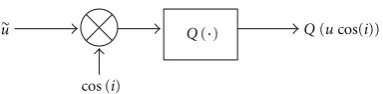
Thus, we can use the following error model for the constant multiplication (22), whereuis the quantization of the input andQ(·) is the truncation operator

We can write

ucos(i)=Q(u·cos(i)) +Δucos(i), (23)

where:Δucos(i) is the truncation error. Thus, we can write

T(k)=

(N−1)/2

i=1

(−1)δ(k,i)Qu(i−k)×cosψ(i)×2α

+Δucosψ(i)×2α

+

(N−1)/2

i=1

(−1)δ(k,i)·Δu(i−k)×cosψ(i)×2α,

T(k)=

(N−1)/2

i=1

+

(N−1)/2

i=1

(−1)δ(k,i)Δucosψ(i)×2α

+

(N−1)/2

i=1

(−1)δ(k,i)·Δu(i−k)×cosψ(i)×2α,

e(k)=T(k)−

(N−1)/2

i=1

e(k)=

(N−1)/2

i=1

+

(N−1)/2

i=1

(−1)δ(k,i)·Δu(i−k)×cosψ(i)×2α. (24)

We will compute the second-order statisticsσ_T2 of the error term. This parameter describes the average behavior of the error and is related to MSE (mean-squared error) and SNR (signal-to-noise ratio).

We assume that the errors are uncorrelated and with zero mean.

We have σ2

T=E

e2₍_k₎

=E ⎧ ⎨ ⎩ ⎡ ⎣(N−1)/2

i=1

+

(N−1)/2

i=1

(−1)δ(k,i)·Δu(i−k)×cosψ(i)×2α ⎤ ⎦

2⎫_⎪ ⎬ ⎪ ⎭

=

(N−1)/2

i=1

EΔ2_u_cos_ψ₍_i₎_×₂_α

+

(N−1)/2

i=1

EΔ2_u₍_i₋_k₎_cos2_ψ₍_i₎_×₂_α_.

(9)

MUX

M

UX

DEMUX ADD

C=0011

Permut and split stage

xa(·)

Add Latch

x(i)

x(_N−1)

Sgn[(−1)i]

C

±

Figure5: The structure of the preprocessing stage for DCT of lengthN=7.

cos (i)

Q(·) Q(ucos(i))

˜

u

Figure6: Truncation error model for a ROM-based multiplication.

It results

σ2

T =

(N−1)/2

i=1 σ2

Δ+σΔ2u

⎛ ⎝(N−1)/2

i=1

cos2_ψ₍_i₎_×₂_α ⎞ ⎠

=(N−1)

2 ·σ

2

Δ+σΔ2u

⎛ ⎝(N−1)/2

i=1

cos2(i×2α) ⎞ ⎠_.

(26)

It can be easily seen that

σ2

T <(N₂−1)·σΔ2+σΔ2u. (27)

We can assume that

σ2

Δ=2 −2M

12 , σ

2

Δx=2

−2L

12 . (28)

We will verify the relation (26) by computer simulation using SNR parameter [31].

In performing the fixed-point round-oﬀerror analysis, we will use the following assumptions:

(i) the input sequencex(i) is quantized usingLbits, (ii) the output of each ROM-based multiplier is

quan-tized usingMbits,

(iii) the errors are uncorrelated with one another and with the input,

(iv) the input sequence x(i) is uniformly distributed between (−1, 1) with zero mean,

(v) the round-oﬀerrors at each multiplier is uniformly distributed with zero mean.

The SNR parameter is computed as

SNR=10 log₁₀σ

2

O

σ2

T, (29)

whereσ2

O is the variance of the output sequence and σT2 is

the variance of the quantization error at the output of the transform.

Using the graphic representation shown in Figures 7–

9, we can see that the computed values agree with those obtained from simulations. Thus, the computed values of SNR have similar values with those computed using relations (26) and (29) represented using snrDfcT plots. InFigure 7, we have shown the dependence of the SNR in our solution on the transform lengthN = 7 andN = 11 as a function of the number of bits L and M used in the quantization of the input sequence and the output of each ROM-based multiplier, respectively, whenM = L. InFigure 8we show the dependence of the SNR for our solution withN =7 as a function ofL, whenM=10, 12, and 14, respectively, and in

Figure 9, we have the same dependence for our solution with the transform lengthN=11.

Thus, we have obtained analytically and we have verified by simulation the dependence of the variance of the output round-oﬀ error with the quantized error of the input sequence σ2

Δx. This is a significant result especially for our

architecture as we can choose appropriately the value of L with L < M. It can be used to significantly reduce the hardware complexity of our implementation as the dimension of the ROM used in the implementation of a multiplier in our architecture is given byM·2Land increases exponentially with the number of bitsLused to quantize the inputu(i) for each multiplier. It can be seen that ifL > M the improvement of the SNR is insignificant. Using these dependences, we can easily choseLsignificantly less thanM. Using the method proposed in [30], where the analysis is made for the direct-form IDCT, we can also obtain for the direct-form DCT, the round-oﬀerror variance (σ_N2)_i

σ2

Ni=(N−1)σR2 for 0≤i≤N−1. (30)

As compared with a direct-form method implementation, known to be robust to the fixed-point implementation and thus used by many chip manufactures [30], the round-oﬀ error variance σ_T2 for the kernel of our solution given by relation (26) is significantly better as we will also see by computer simulations.

(10)

20 30 40 50 60 70 80 90

6 8 10 12 14 16

snrDfcT

SNR

snrDfc7

(a)

30 40 50 60 70 80 90 100

6 8 10 12 14 16

snrDfc11 snrDfcT

SNR

(b)

Figure7: SNR variation function ofMwhenM=L.

6 8 10 12 14 16

45 50 55 60

SNR

snrDfcT 65

70

snrDfc7

(a)M=10

SNR

snrDfcT

6 8 10 12 14 16

40 50 60 70

30 80

snrDfc7

(b)M=12

SNR

snrDfcT

6 8 10 12 14 16

40 50 60 70 80 90

snrDfc7

(c)M=14

Figure8: SNR variation function ofLfor our solution withN=7.

6 8 10 12 14 16

35 40 45 50 55

60 SNR

snrDfc11 snrDfcT

(a)M=10

SNR

6 8 10 12 14 16

snrDfc11 snrDfcT 40

50 60 70

30 80

(b)M=12

SNR

6 8 10 12 14 16

snrDfc11 snrDfcT 30

40 50 60 70 80 90

(c)M=14

(11)

In the case we are using hardwired multipliers instead of LUT based multipliers, there is another error term due to the quantization of multiplier coeﬃcients cos(ψ(i)×2α) of the form

(N−1)/2

i=1

E"u(i−k)2#×Δcosψ(i)×2α2, (31)

where [Δcos(ψ(i)×2α)] is the quantization error of the multiplier coeﬃcient. Thus, the quantization error will be significantly greater for a similar hardwired multiplier based architecture for DCT reported in [32]. It follows that the proposed ROM-based architecture will have better numerical properties as compared with similar hardwired multiplier based architectures for DCT.

Let us also observe that instead of the quantization of the result of relation (22), we can store in the ROMs the rounded value of that result. The rounding error will be less than the truncation error. Thus, the numerical properties of the proposed solution can be further increased.

This result shows that the kernel of our implementation based on (6) has good quantization properties, the error due to a fixed-point representation being small, one of the best results for DCT implementations as will be shown also using computer simulations. Thus, our proposed algorithm and architecture is a very robust solution for a fixed point imple-mentation of DCT. This property can be exploited to further reduce the hardware complexity and the power consumption of the main part of our architecture represented by the above-mentioned kernel. This kernel has the main contribution to the hardware complexity of our architecture and to its power consumption.

5.2. Comparison with Other Relevant Implementations of DCT. In our computer simulations in order to demonstrate the good quantization properties of the proposed solution in comparison with some relevant other ones, we have used several significant parameters as PSNR (peak-signal-to-noise ratio) and the following measures:

(i) overall MSE defined as

MSE= 1

mn

m−1

i=0

n−1

j=0

I f initi,j−Ii,j2, (32)

(ii) peak error defined as

PPE=Max

i

$ Max

j

%

&&_I finiti,j−Ii,j&&. (33)

The numbers for the root of MSE and the value of PPE for diﬀerent values of the word lengthL whenL = M are represented in the Figures10and11.

The values of PSNR are presented inFigure 12in dB for diﬀerent values of the word lengthLwhenM = L. It can be easily seen that the values for PSNR are better for our algorithm than those reported in Hou [29] and for the direct form.

6 8 10 12 14 16

0 0.0025 0.005 0.075 0.01 0.0125 0.015

Bits number (M=L)

HouN=8

PorposedN=7

ProposedN=11

Direct formN=8

Figure10: Mean square error.

8 10 12 14 16

0 0.01 0.02 0.03 0.04 0.05

Bits number (_M=L)

HouN=8

ProposedN=7

ProposedN=11

Direct formN=7

Figure11: Peak error.

The obtained numerical properties of the proposed algo-rithm and its associated VLSI architecture can be exploited to significantly decrease the hardware complexity. Thus, in the proposed architecture, the dimension of the ROMs used to implement the multipliers depends exponentially on the word lengthLused for a fixed-point representation of the input operands. Consequently, we can use small-size ROMs with a short access time to reduce the hardware complexity and to improve the speed. It results that the overall hardware complexity will be significantly reduced due to these good numerical properties and also the power consumption.

(12)

6 8 10 12 14 16 30

40 50 60 70 80 90 100 110

Bits number (M=L)

Hou8 DFC7

DFC11 FD7

Figure12: Peak-signal-to-noise ratio (PSNR).

8 10 12 14 16

0 1000 2000 3000 4000 5000 6000 7000

DCT lengthN

Proposed [16]

[34]

Figure13: ROM words.

First, we can increase the precision used in representing the data in relations (3) and (4) without significantly increasing the hardware complexity.

Then, we can use a high precision for the coeﬃcientsc(i) in the computing of the partial results stored in the ROMs that implement the multiplication with this coeﬃcients.

6. Comparison

The throughput of the VLSI architecture that can be obtained using the proposed algorithm is 2/(N−1) similar to [16,33], but doubled compared to [34]. The pipeline period (average computation time) is (N−1)T/2 as in [16,33] but the clock

7 11 17

24 49 85 92.5 101

DCT length_N

Prososed

[16] [24]

[34]

Figure14: I/O channels.

periodT is significant diﬀerent in these three cases. In the proposed designT=max(TMem,Ta) is significantly less than

in [16], whereT=TMem+Taand in [33], whereT=TMul+

3Taand [34], whereT=TMul+Ta.

We have used the following notations: TMem

-multi-plication time,Ta-adder time, andTMem-access time. Thus,

the proposed design is significantly faster.

If we compare with [24], we can see that (10) can be computed in parallel and thus the throughput can be doubled with respect to [24], where we do not have such a parallelization. Moreover, due to the fact that the two equations have a similar form and the same length, they can be mapped on the same linear systolic array with the ROMs used to implement the shared multipliers. Thus, a significant increase of the throughput can be obtained without doubling the hardware as compared with [24]. The number of control bits is significantly reduced for a double computation (10) as compared with [24].

In order to illustrate the advantages of our proposal, we will consider a numerical example with the lengthN = 37 and the number of bits for the input of multipliersL=10. In this case, the number of multipliers for our proposed solution [16,34] is very small being 2 and 1. Instead, our proposed solution uses 576 words of ROM, [16] uses 1152 words, [28] uses 22 528 words, and [34] have 9 473 000 words. The number of adders is 57 for our solution, 77 for [16], 54 for [33], 107 for [34], and only 20 for [24]. But [24,34] have only a half of the throughput of [16,33] and our solution. The number of bits for I/O channels is 88 for our proposed solution, 107 for [24], and 71 for [16]. In [33,34], we have only 41, respectively, 20 bits for I/O channels.

The comparison between our solution and other VLSI implementations for DCT is presented inTable 1.

Comparing the hardware complexity, we can see from

(13)

Table1: Comparison of hardware complexity of various dct designs.

Structures Multipliers Adders ROM (words) MUXs Cycle-time Throughput ACT I/O channels Proposed 2 3(N+ 1)/2 [(N−1)/2]·2L/2 ₃₍_N₋₁₎ _max(_T

mem,Ta) 2/(N−1) (N−1)T/2 7L+N/2 [16] 2 2N+ 3 [(N−1)/2]·2(L/2+1) ₇_/₂₍_N₋_{1) + 11} _T

mem+Ta 2/(N−1) (N−1)T/2 7L+ 1 [33] (N−1)/2 3(N−1)/2 (N−1) Tmul+ 3Ta 2/(N−1) (N−1)T/2 4L+ 1

[34] 1 3N N(2N/2_{+ 2)} _T

mul+Ta 1/N 2L

[24] (N−1)/2 + 2 (N−1)/2 + 2 2(N+ 1) Tmul+Ta 1/(N−1) (N−1)T 7L+N

for long length N. In Figure 13, we have illustrated the variation of the number of ROM words with respect to the transform lengthNwhenL=10. Also, inFigure 14, we have represented the number of bits used by I/O channels with respect to the transform lengthN when alsoL =12. Note thatLfor other design could be larger as our solution has better quantization properties. It can be seen that the number of bits for the I/O channels in our solution increases slightly with the transform lengthN.

It is also another important aspect to note. The hardware complexity of the preprocessing stage is significantly reduced at about one half in our design as compared with [16] as shown in Figure 5. For relatively, short-length transforms the chip area used by the preprocessing stage represents an important percentage. Also, the hardware complexity of our design of 2 multipliers, 3(N+ 1)/2 adders and (N−1)/2·2L ROM words is significantly reduced as compared with (N− 1)/2 multipliers, 3(N−1)/2 adders in [33].

7. Conclusions

In this paper, a new memory-based design approach that leads to a reduced hardware complexity and a high-throughput VLSI implementation based on a new refor-mulation of DCT having good quantization properties is presented. It uses a parallel VLSI algorithm using parallel cycle and pseudo-cycle convolutions for a memory-based VLSI systolic array implementation. This approach using a new input-restructuring sequence leads to an efficient VLSI implementation with a substantially reduction of the hardware overhead involved by the preprocessing stage of the VLSI array. Moreover, the proposed VLSI algorithm and its associated architecture have good numerical properties that can be efficiently exploited to further reduce the hardware complexity and to obtain a low power implementation. We have shown analytically and by computer simulations that the proposed solution has one of the best quantization prop-erty for DCT that is better than that of the direct-method implementation known to be robust and frequently used in commercial products. The convolution structures can be efficiently implemented using a memory-based systolic array architecture paradigm. The differences in the sign can be efficiently managed using a tag-control scheme. Also, the proposed ROM-based implementation has better numerical properties compared to similar hardwired multiplier-based DCT implementations. It can thus be obtained a new VLSI implementation with a high degree of parallelism and good

architectural topology with a high degree of regularity and modularity and an eﬃcient fixed-point implementation that is well adapted for a VLSI realization. Thus, a new memory-based VLSI systolic array with a high-throughput and a substantially reduced hardware complexity can be obtained.

Acknowledgments

The authors thank the reviewers for their useful comments that have been used to improve the paper. This work was supported by the CNCSIS-UEFISCSU, PNII project ID 310/2008.

References

[1] N. Ahmed, T. Natarajan, and K. R. Rao, “Discrete cosine transform,”IEEE Transactions on Computers, vol. 23, no. 1, pp. 90–94, 1974.

[2] A. K. Jain, “A fast Karhunen-Loeve transform for a class of random processes,” IEEE Transactions on Communications, vol. 24, no. 9, pp. 1023–1029, 1976.

[3] A. K. Jain,Fundamentals of Digital Image Processing, Prentice-Hall, Englewood Cliﬀs, NJ, USA, 1989.

[4] D. Zhang, S. Lin, Y. Zhang, and L. Yu, “Complexity con-trollable DCT for real-time H.264 encoder,”Journal of Visual Communication and Image Representation, vol. 18, no. 1, pp. 59–67, 2007.

[5] Y. Y. Chen, “Medical image compression using DCT-based subband decomposition and modified SPIHT data organiza-tion,”International Journal of Medical Informatics, vol. 76, no. 10, pp. 717–725, 2007.

[6] K. T. Fung and W. C. Siu, “On re-composition of motion compensated macroblocks for DCT-based video transcoding,” Signal Processing: Image Communication, vol. 21, no. 1, pp. 44– 58, 2006.

[7] D. V. Jadhav and R. S. Holambe, “Radon and discrete cosine transforms based feature extraction and dimensionality reduction approach for face recognition,”Signal Processing, vol. 88, no. 10, pp. 2604–2609, 2008.

[8] Z. Wang, G. A. Jullien, and W. C. Miller, “Interpolation using the discrete sine transform with increased accuracy,” Electronics Letters, vol. 29, no. 22, pp. 1918–1920, 1993. [9] Y. S. Park and H. W. Park, “Arbitrary-ratio image

resiz-ing usresiz-ing fast DCT of composite length for DCT-based transcoder,”IEEE Transactions on Image Processing, vol. 15, no. 2, pp. 494–500, 2006.

(14)

[11] K. Mayyas, “A note on “performance analysis of the DCT-LMS adaptive filtering algorithm”,”Signal Processing, vol. 85, no. 7, pp. 1465–1467, 2005.

[12] S. W. A. Bergen, “A design method for cosine-modulated filter banks using weighted constrained-least-squares filters,” Digital Signal Processing, vol. 18, no. 3, pp. 282–290, 2008. [13] B. G. Lee, “Input and output index mappings for a

prime-factor-decomposed computation of discrete cosine trans-form,” IEEE Transactions on Acoustics, Speech, and Signal Processing, vol. 37, no. 2, pp. 237–244, 1989.

[14] X. Shao and S. G. Johnson, “Type-II/III DCT/DST algorithms with reduced number of arithmetic operations,”Signal Pro-cessing, vol. 88, no. 6, pp. 1553–1564, 2008.

[15] P. P. Zhu, J. G. Liu, and S. K. Dai, “Fixed-point IDCT without multiplications based on B.G. Lee’s algorithm,”Digital Signal Processing, vol. 19, no. 4, pp. 770–777, 2009.

[16] D. F. Chiper, M. N. S. Swamy, M. O. Ahmad, and T. Stouraitis, “Systolic algorithms and a memory-based design approach for a unified architecture for the computation of DCT/DST/IDCT/IDST,” IEEE Transactions on Circuits and Systems I, vol. 52, no. 6, pp. 1125–1137, 2005.

[17] C. M. Rader, “Discrete Fourier transform when the number of data samples is prime,”Proceedings of the IEEE, vol. 56, no. 6, pp. 1107–1108, 1968.

[18] Y.-H. Chan and W.-C. Siu, “On the realization of discrete cosine transform using the distributed arithmetic,” IEEE Transactions on Circuits and Systems I, vol. 39, no. 99, pp. 705– 712, 1992.

[19] J. I. Guo, C. M. Liu, and C. W. Jen, “Eﬃcient memory-based VLSI array designs for DFT and DCT,”IEEE Transactions on Circuits and Systems II, vol. 39, no. 10, pp. 723–733, 1992. [20] S. A. White, “Applications of distributed arithmetic to digital

signal processing: a tutorial review,”IEEE ASSP Magazine, vol. 6, no. 3, pp. 4–19, 1989.

[21] H. T. Kung, “Why systolic architectures,”Computer, vol. 15, no. 1, pp. 37–46, 1982.

[22] L. W. Chang and M. C. Wu, “A unified systolic array for discrete cosine and sine transforms,” IEEE Transactions on Signal Processing, vol. 39, no. 1, pp. 192–194, 1991.

[23] S. B. Pan and R. H. Park, “Unified systolic arrays for computation of the DCT/DST/DHT,” IEEE Transactions on Circuits and Systems for Video Technology, vol. 7, no. 2, pp. 413–419, 1997.

[24] J. I. Guo, C. M. Liu, and C. W. Jen, “New array architecture for prime length discrete cosine transform,”IEEE Transactions on Signal Processing, vol. 41, no. 1, pp. 436–442, 1993.

[25] D. F. Chiper, “Novel systolic array design for discrete cosine transform with high throughput rate,” inProceedings of the IEEE International Symposium on Circuits and Systems (ISCAS ’96), pp. 746–749, Atlanta, Ga, USA, May 1996.

[26] S. Yu and E. E. Swartzlander, “DCT implementation with distributed arithmetic,”IEEE Transactions on Computers, vol. 50, no. 9, pp. 985–991, 2001.

[27] M. T. Sun, T. C. Chen, and A. M. Gottlieb, “VLSI implementa-tion of a 16×16 discrete cosine transform.,”IEEE transactions on circuits and systems, vol. 36, no. 4, pp. 610–617, 1989. [28] P. K. Meher, “Unified systolic-like architecture for DCT

and DST using distributed arithmetic,”IEEE Transactions on Circuits and Systems I, vol. 53, no. 12, pp. 2656–2663, 2006. [29] H. S. Hou, “A fast recursive algorithm for computing the

discrete cosine transform,” IEEE Transactions on Acoustics, Speech and Signal Processing, vol. 35, no. 10, pp. 1455–1461, 1987.

[30] I. D. Yun and S. U. Lee, “On the fixed-point error analysis of several fast IDCT algorithms,”IEEE Transactions on Circuits and Systems II, vol. 42, no. 11, pp. 685–693, 1995.

[31] C. Y. Hsu and J. C. Yao, “Comparative performance of fast cosine transform with fixed-point roundoﬀerror analysis,” IEEE Transactions on Signal Processing, vol. 42, no. 5, pp. 1256– 1259, 1994.

[32] D. F. Chiper, M. N. S. Swamy, and M. O. Ahmad, “An eﬃcient unified framework for implementation of a prime-length DCT/ IDCT with high throughput,”IEEE Transactions on Signal Processing, vol. 55, no. 6, pp. 2925–2936, 2007. [33] C. Cheng and K. K. Parhi, “A novel systolic array structure for

DCT,”IEEE Transactions on Circuits and Systems II, vol. 52, no. 7, pp. 366–369, 2005.