Transformation.
Thesis by Bharat Penmecha
In Partial Fulfilment of the Requirements for the Degree of
Doctor of Philosophy
California Institute of Technology Pasadena, California
2013
Acknowledgements
I couldn’t thank Kaushik enough for believing in me and giving me an opportunity to work with him. It has been quite a journey since the summer of 2008 and I wouldn’t have achieved whatever I have in my PhD without his unconditional support. I thank him most for giving me the room to explore and learn on my own and develop my research aptitude. His positive visage, emphasis on seeking insight without getting lost in finer details and boldness in looking at traditional ideas from a fresh perspective will stay with me for the rest of my life. I thank Prof. G. Ravichandran for all the advice and support he has extended over the years, especially for offering me support through Teaching Assistantship for Ae/ME 102 over many terms and serving on my thesis committee. I thank Prof. Michael Ortiz for agreeing to serve as my committee chair and offering feedback on my thesis. He has been a great source of inspiration for pursuing Mechanics. I thank Prof. Dennis Kochmann for serving on my committee and sharing his experience.
I have had some great colleagues at Caltech. I should start by thanking Dr. Phanish Suryanarayana, my office mate for three years for being the go-to guy on many a topic. It has been a wonderful experience to interact with the members of Kaushik’s and Ravi’s groups over the years - Andrew Richards, Dr. Zubaer Hossain, Dr. Saurabh Puri, Srivatsan Hulikal, Ha Jiang, Cindy Wang, Dr. Pierluigi Cesana, Farshid Roumi, Chris Kovalchik, Justin Brown, Jacob Notbohm, Aaron Stebner and Aaaron Albretch.
Endrizzi - who make it special.
I have had the pleasure of making many friends outside work at Caltech which made the place even more special. I am lucky to have had some great room-mates - Prakhar Mehro-tra, Navneet Narayanan, Ajay B.H, Manav Malhotra - during my memorable stay in the Catalina apartments. Nakul Reddy, Raviteja Sukhavasi, Naresh Satyan, Vahe Gabuchian, Jayakrishnan Unnikrishnan, Rangoli Sharan, Kaushik Sengupta, Dr. Sujit Nair have been great company.
I extend my gratitude to Amith Pinapala, my closest friend of many years, whose guidance and friendship has helped me steer through difficult times. I much appreciate him pointing me in a sensible direction whenever I was at a crossroads.
Special thanks to Piya Pal who has been a significant part of my life in the last few years for all the care, support and inspiration. She is a very special human being and I am grateful to destiny for making her a part of my life.
Abstract
A large number of technologically important materials undergo solid-solid phase transforma-tions. Examples range from Ferroelectrics (transducers and memory devices), zirconia (Thermal Barrier Coatings) to nickel superalloys and (lithium) iron phosphate (Li-ion bat-teries). These transformations involve a change in the crystal structure either through dif-fusion of species or local rearrangement of atoms. This change of crystal structure leads to a macroscopic change of shape or volume or both and results in internal stresses during the transformation. In certain situations this stress field gives rise to cracks (tin, iron phosphate etc.) which continue to propagate as the transformation front traverses the material. In other materials the transformation modifies the stress field around cracks and effects crack growth behaviour (zirconia, ferroelectrics). These observations serve as our motivation to study cracks in solids undergoing phase transformations. Understanding these effects will help in improving the mechanical reliability of the devices employing these materials.
only distorts it from its mean straight shape. We then consider the stability of the parallel system of cracks against period doubling instability commonly seen in thermal cracking. After performing a linear stability analysis we conclude that the system of cracks is stable against this bifurcation. We go on to ascertain this conclusion by performing numerical simulations using finite elements. Finally, using arguments based on energy balance we derive an optimal spacing for the parallel system of cracks. From this analysis the following picture of crack growth emerges - for a given transformation strain parallel cracks initiate and assume a uniform spacing after a transient stage, grow all the way till their tips cross over the phase boundary and continue to grow as the phase boundary propagates at a uniform spacing without any instabilities.
Second, we model the effect of the semiconducting nature and dopants on fracture in ferroelectric perovskite materials, particularly barium titanate (BaTiO3). Traditional
Contents
Acknowledgements iv
Abstract vi
1 Introduction 1
1.1 Solid-solid phase transformations . . . 1
1.2 Fracture and phase transformations. . . 2
1.3 Organization . . . 3
2 Directional Edge Crack Growth Due to a Phase Transformation 7 2.1 Introduction. . . 7
2.2 Overall setting . . . 11
2.2.1 Dissipation inequality and equilibrium . . . 11
2.2.2 Propagation laws . . . 14
2.2.3 Stability of a propagating system of cracks . . . 15
2.3 Stress analysis . . . 16
2.3.1 Stress due to a phase boundary . . . 16
2.3.2 Stress due to the interaction of cracks with a phase boundary . . . . 19
2.4 Phase boundary. . . 22
2.5 Crack propagation . . . 24
2.5.1 Cracks with uniform spacing and length . . . 24
2.5.2 Stability against period doubling . . . 28
2.6 Numerical study . . . 29
2.7.1 One flaw in a unit cell . . . 32
2.7.1.1 Stationary phase boundary . . . 32
2.7.1.2 Moving phase boundary . . . 33
2.7.2 Multiple flaws in a unit cell . . . 34
2.8 Conclusions . . . 36
2.9 Future Directions . . . 36
3 Effect of Space Charges on Fracture in Ferroelectric Peroskites 38 3.1 Introduction. . . 38
3.2 Ferroelectric perovskites . . . 41
3.3 Fracture behaviour of ferroelectric perovskites . . . 44
3.3.1 Experiments on fracture of ferroeletrics . . . 45
3.3.2 Modelling and simulation . . . 47
3.4 Semiconducting nature of Ferroelectric perovskites . . . 50
3.4.1 Semiconductor physics . . . 50
3.4.2 Defects in perovskites . . . 53
3.5 Phase field model . . . 55
3.5.1 Kinematics . . . 56
3.5.2 Rate of dissipation . . . 56
3.5.3 Governing equations . . . 61
3.5.4 Crack surface boundary conditions . . . 62
3.6 Constitutive relations . . . 65
3.7 Implementation . . . 69
3.7.1 Finite element formulation . . . 72
3.8 Results. . . 75
3.8.1 No space charge,ρ= 0 . . . 77
3.8.2 n-type dopants . . . 78
3.8.3 p-type dopants . . . 79
3.8.4 Discussion. . . 79
3.9.1 Results . . . 81
3.10 Driving force on the crack : The J-integral. . . 82
3.10.1 Results of J-integral . . . 84
3.11 Summary and conclusions . . . 84
A Appendices 92 A.1 Stress field of a shallow phase boundary . . . 92
A.2 Solution to the integral equations . . . 94
A.3 Integral identities . . . 97
A.4 Optimal orientation of phase boundary. . . 98
A.5 Driving force on a phase boundary . . . 100
A.6 Divergence free property of augmented energy momentum tensor . . . 100
A.7 Domain integral for evaluating driving force, J . . . 102
List of Figures
1.1 Cubic to monoclinic transformation of Nitinol. Reproduced from [64] . . . . 2 1.2 Cracks resulting from phase transformation. (a) SEM micrographs of polished
surfaces of CsH2PO4 above the phase transition temperature [65]. (b) SEM
image of a partially delithiated LiFePO4 single crystal [119].(c) Cracked single
crystal BaTiO3after subjecting to cyclic electric loading [16] . . . 4
2.1 Directional crack growth seen in experiments: (a) Phase transformation
in-duced cracks in CsHSO4 [65]. (b) Parallel edge cracks in a glass plate due to a
sharp thermal gradient [88]. (c) Edge cracks due to drying in a film of sol-gel
[46] . . . 8 2.2 A body with a crack and a phase boundary. . . 11 2.3 Geometry of the problem showing the phase boundary, free surface and cracks,
and the partition into simpler problems used for stress analysis. . . 19 2.4 Unit cell of width 2b containing two cracks, chosen for the analysis . . . 22 2.5 (a) Normalized driving force on the phase boundary due to the presence of the
cracks over one unit cell containing a single crack. Negative values indicate
force towards the cracks. The mean value over one unit cell is zero. (b)
The equilibrium shape of the phase boundary. In both figures, we use b =
2.6 The stress intensity factor experienced by the cracks of uniform length h and
spacing b due to the phase transformation. (a) The variation of the stress
intensity factor with crack length. The vertical dashed line indicates the
posi-tion of the phase boundary (b= 10mm, L= 15mm). (b) The stress intensity
factor for various crack-spacings (L= 15mm). (c) The normalized stress
in-tensity factor for various crack-spacings (L = 15mm). (d) The normalized
stress intensity factor for various positions of the phase boundary (b= 10mm). 25
2.7 Variation of the normalized stress intensity factors (N =K/σ0
√
2πb)
experi-enced by the two cracks when the length of one is varied while the that of the
other is held fixed. Here, the phase boundary position is L= 15mmindicated
by the dotted vertical line while the crack spacing is b = 10mm. Crack #1
has a length h1= 15.4mmwhile crack # 2 varies in the range [14mm,16mm]. 28
2.8 Unitcell geometry and boundary conditions.. . . 30 2.9 Traction-separation law with linear damage evolution. . . 31 2.10 Comparison between predictions of theory and numerical simulation. The
red points represent the normalized critical stress intensity Ncand final crack
length for various transformation strains computed numerically. The blue
curve shows the normalized stress intensity as a function of normalized crack
length. Note that cracks do not grow when Nc> N∞ and grow to the phase
boundary when N < N∞ showing consistence between theory and numerical
simulation. (b = 0.1mm, L = 0.15mm). The cross-hair on the left indicates
the initial flaw. . . 32 2.11 Crack growth with a moving phase boundary. Left: The crack length as a
function of the phase boundary position for three different values of
transfor-mation strain (or equivalently ∆T). Right: Three snap-shots for εo= 0.24%.
2.12 Crack growth with two cracks in a unit cell for varying transformation strains.
(a) Three snap-shots with transformation strain of 0.16% shows neither crack
grows. (b) Three snap-shots with transformation strain of 0.184% shows the
one crack grows along with the phase boundary. (c) Three snap-shots with
transformation strain of 0.22% shows the both cracks grow along the grows
along with the phase boundary. The flaw spacing isb= 0.1mmand the critical
flaw spacing for crack growth at the applied strain based on Nf law are: (a) ∞
(b) 0.17mmand (c) 0.056mm . . . 34 2.13 Crack growth with four cracks in a unit cell at various transformation strains.
Crack length vs interface position for (a) εo = 0.16% (b) εo = 0.184% (c)
εo= 0.22%. The flaw spacing is b= 0.1mm.. . . 35
3.1 Cracks in piezoelectric actuators. (a) Multilayer actuator (b) Electric discharge 39
3.2 Perovskite structure of BaTiO3 in the cubic and tetragonal state. Reproduced
from [15]. . . 42 3.3 (a)Six variants of BaTiO3. (b) Polarized light optical micrographs of domain
patterns in BaTiO3single crystal [16].(c) Domains of variants in a BaTiO3crystal
[48]. . . 43 3.4 Switching of BaTiO3 unitcell under electromechnaical loading. Reproduced
from http://www.ae.utexas.edu/ landis/Landis/Research.html. . . 44 3.5 Evolution of domain switching near a crack tip in poled PMN-PT(62-38) single
crystal under negative electric fields. Reproduced from Jiang et.al. [51]. . . . 47 3.6 (a) Topographic image and (b) surface potential image of the
indentation-pre-cracked BaTiO3 single crystal. Reproduced from Sun et.al. [105].. . . 47
3.7 Band diagram of crystalline solids. . . 51 3.8 Band diagrams of extrinsic semiconductors. . . 52 3.9 Metal, n-type Semiconductor interface. (a) Before contact. (b) After contact
showing the depletion layer and band bending. . . 53 3.10 Ferroelectric domain with a crack subject to tractions and external electric
3.11 Landau-Ginzburg multiwell potential, Wp. (a) Four-well structure, (b)
Con-tour plot of the wells. . . 66 3.12 Variation of space charge density with electric potential at thermal equilibrium
with n-type dopants, T = 300K, Nd= 1024, Na= 0, Ef m=−5.3eV.. . . . . 68
3.13 Variation of space charge density with electric potential at thermal equilibrium
with p-type dopants, T = 300K, Na= 1024, Nd= 0, Ef m=−5.3eV.. . . 68 3.14 Mesh used for the simulations and boundary conditions. . . 76 3.15 Polarization evolution for σo = 0, φo= 0.1. nrepresents the time step. . . . 86 3.16 Results for σo = 0, φo = 0.1.(a) Polarization domains around the crack, (b)
σ22, (c) Electric potential, φ. . . 87
3.17 Results for n-type dopants at σo = 0, φo = 0.1, Nd = 1024 (a) Polarization
domains around the crack, (b)σ22, (c) Electric potential,φ, (d) Space Charge,
ρ. . . 88 3.18 Results for p-type dopants at σo = 0, φo = 0.1, Nd = 1024. (a) Polarization
domains around the crack, (b) σ22, (c) electric potential,φ, (d) space charge, ρ. 89
3.19 Results from the 1-D model at different L. Nd= 1024, Na= 0. Left columns
showsp (blue) andφ(green). The right column shows ρ. . . 90 3.20 Variation of J with φo for different doping. σo = 0. . . 91 3.21 Variation of J with φo for different doping. σo = 0−1.. . . 91
A.1 Geometry of perturbed interface and the sub-problems for superposition. . . 92 A.2 Notation for domain integral formulation to evaluate the driving force on a
Chapter 1
Introduction
1.1
Solid-solid phase transformations
Solid-solid transformations are phase transformations when a solid in a parent phase under-goes a transformation to another solid with a different crystal structure. A good example is the popular ferroelectric material barium titanate, BaTiO3, used widely in transdcuing
applications. Above its Curie temperature of, Tc= 120oC, BaTiO3exists in a state with a
cubic unit cell. Upon cooling, the cubic unit cell transforms into tetragonal. Other popular examples are the Martensitic transformation of iron and shape memory alloys like nitinol (NiTi), transformation between iron phosphate and lithium iron phosphate upon insertion and removal of lithium ions, the protonic transformation of solid acid materials, and the transformation of zirconia.
Transformations which involve long range diffusion of species are termed diffusional. Transformations in which there is a change in lattice structure only through a local rear-rangement of the species are termed diffusionless or martensitic transformations. These rearrangements are small, usually less than the interatomic distances, and the atoms main-tain their relative relationships. A good example is the transformation of the popular shape memory alloy nitinol which undergoes a transformation from a cubic lattice to monoclinic, see Figure1.1. The change in the lattice structure due to transformation is characterized by the transformation or Bain strain which represents the stress free strain of the transformed lattice of the material with respect to the parent lattice.
technolog-Figure 1.1: Cubic to monoclinic transformation of Nitinol. Reproduced from [64]
ical importance. The martensitic transformation of steel is responsible for producing steel of high strength. Shape memory alloys due to their superelasticty and shape memory prop-erties have been the basis for high power density actuators in the aviation and automotive industries and numerous applications in the medical device industry ranging from dental braces to stent grafts for minimally invasive endovascular procedures. Rechargeable battery technology using lithium iron phosphate as the cathode material have been found to have greater life span, higher power density and safer to operate. This battery technology holds promise for use in hybrid vehicles and consumer electronics. Solid acid compound materials, cesium hydrogen phosphate and cesium hydrogen sulphate undergo a transformation into a phase with high proton conductivity which make them potential fuel cell electrolyte materi-als. Ferroelectric perovskite materials like BaTiO3and PZT have long been used in sensing
and actuating applications in their polar state. Through intelligent domain engineering high strain actuators are being developed which take advantage of the strain produced through domain switching.
1.2
Fracture and phase transformations
cracks as the transformation proceeds further.
Cracks arising out of phase transformations have been observed in several instances in-volving brittle materials. Figure (1.2) shows various instances where transformation leads to fracture. Cracks have been observed to initiate near the embedded electrodes in PZT multilayer piezoelectric actuators during the poling process and seen to grow subsequently ultimately leading to electric discharge. Electrodes used in Li-ion batteries have been known to develop cracks during the cyclic lithiation and de-lithiation which leads to fade in the capacity. Cycling of solid acid material, CsH2PO4, due to the incompatibility of
transfor-mation strain, leads to a network of microcracks which is undesirable for the functioning of the electrolyte.
Understanding the mechanics behind the growth of cracks arising out of phase trans-formations would help in improving the reliability of the promising technologies based on phase transforming materials. This serves as the motivation for this thesis. Typically in these materials there is other physics also at work. For example ferroelectric and piezo-electric materials involve a coupling between piezo-electrical and mechanical fields, Lithium iron phosphate based electrode involves diffusion of Li-ions , and solid acid materials involve proton transport. So the mechanics of cracks arising in these instances is coupled to the additional physics. As a result a holistic theory of the interplay between cracks and phase transformations is quite difficult to establish and so each case warrants a subjective analysis.
1.3
Organization
(a) (b)
(c)
Figure 1.2: Cracks resulting from phase transformation. (a) SEM micrographs of polished surfaces of CsH2PO4 above the phase transition temperature [65]. (b) SEM image of a
partially delithiated LiFePO4 single crystal [119].(c) Cracked single crystal BaTiO3after
subjecting to cyclic electric loading [16]
uniform spacing without any instabilities.
dimensional simulations using a domain integral approach.
Chapter 2
Directional Edge Crack Growth
Due to a Phase Transformation
2.1
Introduction
Solid to solid phase transformations lie at the heart of a number of important technological applications. Such transformations are characterized by a change of crystal structure which manifests itself as a change of shape and volume as one phase transforms into another. Therefore, the process of transformation during which the two phases co-exist can give rise to stresses. These stresses in turn can lead to internal twinning, plasticity and incoherent interfaces, or fracture. Phase transformation induced fracture motivates the current work. Tin pest is a well-known example of such a phenomenon. Often, phase boundaries nucleate on a free surface and propagate into the body leaving a wake of fractured materials behind it. This is known as directional cracking or directional crack growth.
Directional crack growth is observed in a wide range of situations involving inhomoge-neous shrinkage or expansion besides phase transformations, especially as a temperature or concentration gradient results in gradients of stress-free strain. Basalt columnar formations in solidifying and cooling lava [28], cracking in glass due to thermal shock [9] are two ex-amples involving a temperature gradient. Cracks seen in mudflats [28], cracking of Li-ion battery anodes [38] are examples which involve concentration gradients.
(a)
growth direction
(b) (c)
Figure 2.1: Directional crack growth seen in experiments: (a) Phase transformation induced cracks in CsHSO4 [65]. (b) Parallel edge cracks in a glass plate due to a sharp thermal
gradient [88]. (c) Edge cracks due to drying in a film of sol-gel [46] .
CsHSO4 [65], drying of aqueous sol-gel films [46], and thermal cracking of glass [88]. This
can happen in both bulk (CsHSO4) as well as in thin specimens (sol-gel films, glass).
behaviour 2) In the tunnelling cracks case the spacing scales with the film thickness and is weakly dependent of crack length.
However, no such instability is observed when the change of stress-free strain is sharp or occurs with a very high gradient. This was noted in Bazant et.al [13], where a finite element study of thermal cracks did not reveal a bifurcation for sharp temperature profiles. Shorlin et.al [97] studied shrinkage cracks that form when a thin layer of alumina/water slurry dries. A set of parallel cracks with uniform spacing form and grow in a directional manner with the sharp drying front. Once established, the spacing does not change. Allain and Limat [5] as well as Pauchard et.al [81] make similar observations with the drying of colloidal suspensions. Rosin and Perrin [88] drove a a thin glass plate at a constant velocity between two thermal baths at different temperatures, and observed stable crack growth when the velocity established a sharp gradient. They also point out the fact that the crack fronts in the middle of the plates had their tips at the same horizontal level establishing a uniform crack front.
A number of modelling approaches have been adopted to simulate the parallel crack patterns seen in thermal shock experiments [8, 40, 88] and drying films [5, 97]. Fracture mechanics combined with static crack finite element calculations were used in [73,12, 13], the boundary element method in [10, 7], peridynamics in [56], a variational fracture ap-proach [62] and spring network models [44]. Jagla [49] presents a theory based on energy minimization to explain the observations in thin drying layer of materials. He also presents arguments for cracks attaining a uniform spacing.
show that cracks nucleate when the phase boundary has propagated a certain distance Lcr
(see Figure 2.6) from the free edge. The cracks have uniform spacing b? (see Eq. (2.5.3)),
and nucleate with initial length slightly larger thanLcr. Subsequently all the cracks
prop-agate with the propagating phase boundary in such a manner that the spacing remains uniform and the tips reach just beyond the phase boundary. The choice for uniform spacing is based on the observations both in experiment [88, 82] and simulations [49, 62, 10, 56], where randomly spaced cracks, after a transient growth phase readjust the spacing between them and establish a uniform spacing either by merging with adjacent cracks or stopping to grow.
Our analysis is limited by a few important assumptions. First, we assume that the elastic modulus and fracture toughness of both phases are the same. This enables us to use superposition in our stress analysis and avoid the issues of crack propagation along the phase boundary and pinning typically associated with heterogeneous materials. The problems of cracks propagating normal to an interface separating heterogeneous media have been considered in [47]. We also assume that the modulus is isotropic. While these assumptions are reasonable in thermal/concentration gradient induced cracks, they may not be in phase transitions. Still we believe that the results we present are qualitatively meaningful. Second, we assume that the phase boundary is roughly parallel to the free edge. Again, this assumption is reasonable in thermal/concentration gradient induced cracks, it may not be in phase transitions. In the latter, the phase boundary is a very specific interface which may or may not coincide with the free edge. However, the situation analysed here constitutes the worst case scenario. Third, our analysis is limited to uniformly spaced potential cracks. Our analysis shows that there is a particular spacing that is preferred. Further, this preferred spacing is determined by the transformation strain alone, and that this spacing is stable against various instability. Therefore, we expect that the mode-II loading generated by the non-uniform spacing would result in crack deviation and merging eventually resulting in a uniform spacing.
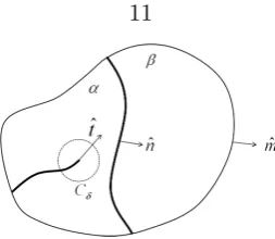
Figure 2.2: A body with a crack and a phase boundary.
2.3.1the state of stress that can result from a phase transformation, and identify the specific conditions that cause a single tensile principal stress that in turn can lead to parallel cracks. We specialize to the problem of interest in Section 2.3.2. We consider a phase boundary roughly parallel to the free edge propagating into a solid and an array of parallel cracks perpendicular to the edge propagating into the solid in the wake of the phase boundary. Section2.3.2derives the resulting stresses. We study how the phase boundary propagation is affected by the cracks in Section2.4. We show that cracks create local perturbations, but does not affect the overall propagation of the phase boundary.
The main analysis of crack propagation is presented in Section 2.5. We begin with the study of cracks of uniform spacing and length in Section 2.5.1, and then study cracks of uniform spacing but alternating length in Section 2.5.2. These allow us to draw the conclusions describe above. We confirm these conclusions through numerical simulation in Sections 2.6 and 2.7. We conclude in Section 2.8 and provide ideas for future work in Section2.9.
2.2
Overall setting
2.2.1 Dissipation inequality and equilibrium
Consider a body Ω consisting of two phasesαand β occupying complementary sub-regions Ωα and Ωβ as shown in Figure 2.2. These phases are separated by a phase boundary S,
δ and consider only the region Ωδ = Ωα\Cδ. There is an external traction t0 acting on a
part Ωt of the boundary of Ω, and displacement is specified on the rest of the boundary.
The total energy of the system is given by,
Πδ(u,Γ,S) =
Z
Ωδ
ψα(∇u)dx+
Z
Ωβ
ψβ(∇u)dx−
Z
Ωt
to.uds, (2.2.1)
where
ψα(ε) =
1 2(ε−ε
?)
·C(ε−ε?) +ω,
ψβ(ε) =
1
2ε·C, ε (2.2.2)
where C is the elastic modulus assumed to be uniform across the phases, ε? is the
trans-formation strain (stress-free strain or eigenstrain) and ω is the chemical potential. The assumption of equal elastic modulus is essential as it allows various applications of the prin-ciple of superposition in what follows. Further, we assume that this uniform modulus is isotropic and the transformation strainε?is diagonal (the latter is without loss of generality
by a change of coordinates). We use the notation ψ =χαψα+ (1−χα)ψβ, where χα
rep-resents the indicator function over Ωα, to represent the elastic energy density of the body.
We adopt the following notation going further, u is the particle displacement, u particle velocity, a= ˙aˆtis the crack tip velocity, v is the phase boundary velocity, vn=v.ˆk is the normal velocity of the phase boundary, ˆc represents the normal to the curve Γ, the crack surface.
Above, we have neglected surface energy along the crack faces, and interfacial energy on phase boundary. We note that the former does not change the results since it can easily be accounted for in the crack propagation criterion. Regarding the latter, we are interested in situations where the elastic energy is significant so that the phase boundaries are almost planar.
dissipation in the body under the loading and the evolution of the phase boundary and the cracks.
D=F − E ≥0, (2.2.3)
where F represents the rate of external work and E is the rate of change of energy of the body Ω. The rate of external work is given by
F =
Z
∂Ωt
to.uds, (2.2.4)
the rate of change of energy of the body is
E = d dt
Z
Ωt
ψdx. (2.2.5)
Assuming no flux on the boundary ∂Ωt, the transport identity (A.3.3), leads to
E =
Z
Ω\Cδ
˙
ψdx−lim
δ→0
Z
∂Cδ
ψ(a.ˆn)ds−
Z
S
[[ψ]]vnds. (2.2.6)
Expanding the first term and using the divergence theorem (A.3.6) leads to
E=
Z
∂Ωt
∂ψ
∂ε.u.mdsˆ −
Z Ωt ∇. ∂ψ ∂ε
.udx−lim
δ→0
Z
∂Cδ
ψ(a.ˆn) +∂ψ ∂εu.ˆn
ds
−
Z
S
[[ψ]]vnds−
Z
S
∂ψ ∂ε.u
.ˆkds−
Z
Γ
∂ψ ∂ε.u
.ˆcds. (2.2.7)
The above equation can be simplified further using the following
[[αβ]] = [[α]]hβi+ [[β]]hαi, σ= ∂ψ
∂ε, (2.2.8a) [[u]] +vn[[∇uT]].kˆ= 0 on S, u=∇u.a on ∂Cδ. (2.2.8b)
velocitya. Substituting (2.2.8) into (2.2.7), the expression for Dtakes the form
D=
Z
Ωt
∇.σ.udx+
Z
∂Ωt
(to−σ.m)ˆ ds+ lim δ→0
Z
∂Cδ
ψ(a.ˆn) +∇uTσ.ˆn.a
ds
+
Z
S
[[ψ]]−[[∇uT.k]]ˆ hσ.kˆiv nds+
Z
S
[[σ.ˆk]]huids+
Z
Γ
[[σ.ˆc]].uds. (2.2.9)
Note that the terms contributing to the dissipation are arranged in conjugate pairs - gener-alized velocity times a conjugate force. Using the arguments presented in [22], equilibrium under isothermal conditions, assuming traction free crack faces leads to
∇ ·σ= 0, σ.mˆ =to on ∂Ωt [[σ]]ˆk= 0 on S, σ =
C(ε−ε?) in Ωα
Cε in Ωβ
. (2.2.10)
2.2.2 Propagation laws
The driving forces conjugate to crack propagation and phase boundary propagation are respectively
da = lim δ→0
Z
∂Cδ
ˆ
t·(ψI − ∇uTσ).ˆnds , (2.2.11) dS = k.[[ψIˆ − ∇uTσ]].kˆ= [[ψ]]− hσi: [[ε]]. (2.2.12)
where ˆtis the tangent to the crack at the tip. For the energy density as in (2.2.2) and for an boundary moving into the theβ−phase, the expression for the driving force reduces to
dS=hσi:ε?−ω, (2.2.13)
The propagation of the cracks and the interface conditions follow the kinetic relations
˙
a=fa(da) vn=fS(dS), (2.2.14)
whereais the crack length andvnis the normal velocity of the phase boundary. We assume
rate-independent kinetic relations :
da ≤Gc, a˙ = 0 if da< Gc, and ˙a≥0 ifda=Gc , (2.2.15)
|dS| ≤dc, vn= 0 if |dS|< dc, and dSvn≥0 if|dS|=dc, . (2.2.16)
Above, Gc is the critical energy release rate and dc is the critical driving force for
interface propagation. We also restrict ˙a≥0 to prevent crack healing.
2.2.3 Stability of a propagating system of cracks
Consider a loading system where two cracks propagate with a smooth time history a1(t)
and a2(t) such that it satisfies the condition (cf. (2.2.15))
d1
a(a1(t), a2(t)) =d2a(a1(t), a2(t)) =Gc. (2.2.17)
Now assume that beginning at timet=t?, we have an alternate smooth crack historyb
1(t)
and b2(t) with ˙bi ≥0 consistent with the loading and propagation criterion :
d1a(b1(t), b2(t))≤Gc, d2a(b1(t), b2(t))≤Gc. (2.2.18)
Subtracting (2.2.18) from (2.2.17) and expanding around t = t?, we find the necessary
condition for bifurcation to be
2
X
j=1
where
Hij =
∂di a
∂aj
(a1(t?),a2(t?))
. (2.2.20)
Note that this condition is somewhat subtle since we require ˙ai,b˙i to be non-negative. In
other words, one can have a singular Hessian H, but still be stable because the criticality occurs along inadmissible crack histories.
This analysis, consistent with those in [12] and [74], assumes that the crack paths and crack trajectories are differentiable. However we note that this may not always be the case [19] for rate-independent laws.
2.3
Stress analysis
2.3.1 Stress due to a phase boundary
We begin by studying the nature of stresses that arise as a consequence of the phase tran-sition. This depends on the elastic moduli of the two phases, the transformation strain as well as the microstructure (i.e., the geometric arrangement of the two phases). In many structural phase transitions, the microstructure that arises is the one that minimizes the free energy of the system. This in turn is dominated by the strain energy for large enough transformation strains. The problem of computing the optimal microstructure remains open in general (see for example Chenchiah and Bhattacharya [21]). However, when both phases have the same elastic modulus as assumed in this work, Kohn [57] has shown that the optimal arrangement is laminates with a specific interface normal.
If the transformation strain is a symmetrized rank-one matrix, i.e.,ε?= γ
2(ˆn⊗mˆ + ˆm⊗n)ˆ
for some scalar γ and unit vectors ˆn,m, then the two phases can co-exist in a stress-freeˆ manner with an interface with normal ˆnor ˆm. If,ε? is not of this form, then Kohn [57] has
shown that the the best possible interface is one that affords the best approximation ofε?
to a symmetrized rank-one matrix. Specifically, let ˆn, ˆm solve the variational problem:
γ = max
ˆ
n,mˆ
(ˆn⊗mˆ + ˆm⊗ˆn)·Cε?
((ˆn⊗mˆ + ˆm⊗n)ˆ ·C(ˆn⊗mˆ + ˆm⊗ˆn))1/2
Then, the interface between the two phases is either ˆn or ˆm. Further, the jump in strain across the interface is
[[ε]] = γ
2(ˆn⊗mˆ + ˆm⊗n)ˆ , (2.3.2) so that jump in stress across the interface is
[[σ]] =C γ
2 (ˆn⊗mˆ + ˆm⊗n)ˆ −ε
?. (2.3.3)
For specificity, let us assume that the interface normal is ˆn. Then, traction continuity requires that [[σ]]ˆn= 0. It follows that the normal to the interface is one of the principal axes of the stress jump with principal value zero. In other words, the state of stress resulting from the phase transformation is at most biaxial along two normal directions that lie on the phase boundary.
If both of these are tensile, then we expect to see a network of cracks like in basalt and if both are compressive, we may see interfacial fracture. However, if exactly one of them is tensile, we expect to see parallel cracks of the type we analyse here. This happens exactly when the product of the two principal stresses is non-positive. However, notice that this product is also the determinant of the projection of the stress to the plane of the interface. Putting this together, we conclude that we expect to see parallel cracks when
ˆ
n·cof([[σ]])ˆn≤0, (2.3.4)
where cof( ) represents the cofactor, [[σ]] is given by (2.3.3), andγ,ˆn,mˆ are given by (2.3.1). To illustrate this condition, let
ε?=
ε∗
1 0 0
0 ε∗2 0 0 0 ε∗3
. (2.3.5)
We effectively have two situations.
the metallic, white β form of tin transforms to the brittle, grey α form upon cooling below 13.2◦C. The transformation strain from α to β is characterized by ε∗1 = ε∗2 = −0.113, ε∗3=−0.0204, [84]. Let ˆei, (i= 1,2,3) denote the principal directions ofε∗.
In this case, the optimal normal according to (2.3.1) is any vector in the ˆe1−eˆ2plane.
If we choose it to be ˆe1, then the jump in stress components is
[[σ22]] =−E
ε∗3+νε∗2
1−ν2 , [[σ33]] =−E
ε∗2+νε∗3
1−ν2 . (2.3.6)
Since all the strains are negative, the stress jump has two positive principal values. One would expect a network of cracks similar to mud-cracking unless we are in plane stress.
We note that the case 0 < ε∗
1 < ε∗2 < ε∗3 is essentially the same with the roles of the
two phases and the sign of the stresses reversed. • Case 2: ε∗
1 < ε∗2 <0< ε∗3. The intercalation phase transition in LiFePO4is an example
with ε∗1 =−0.056, ε2∗ =−0.0434, ε∗3 = 0.013 [66]. In this case, the interface normal depends on the specific details of the transformation strain and elastic modulus. For the values of the transformation and elastic moduli for LiFePO4, the normal happens
to be ˆe1, and this is in agreement with observations. Further, the jump in stress is
again given by (2.3.6). It is readily verified that the jumps have opposite signs. Thus, we have only one tensile principal stress, and we anticipate the formation of parallel edge cracks as seen in [118, 38]. To analyse crack formation and growth we confine the analysis to the plane perpendicular to the crack fronts.
We note that the case ε∗1 <0 < ε∗2 < ε∗3 is essentially the same with the roles of the two phases and the signs of the stress reversed.
In summary, we expect to see an array of parallel cracks in Case 2.
Another situation in which we expect to see an array of parallel cracks is in plane stress. When the in-plane components of transformation strainε∗
1, ε∗2 are opposite in sign, the two
(A)
(B)
L
+
+
hi
~
~
(C)
xy
Figure 2.3: Geometry of the problem showing the phase boundary, free surface and cracks, and the partition into simpler problems used for stress analysis.
eigenvalue and the state of stress in theαphase is uniaxial. This is the situation in LiFePO4
flakes often used in batteries.
2.3.2 Stress due to the interaction of cracks with a phase boundary
We now specialize to the geometry of interest and to two dimensions. We seek to address nucleation and growth of cracks when the interface is close to a free edge. This interface may represent a phase boundary as discussed in the previous section, or also a region of high gradient of temperature or concentration separating regions of uniformity. We assume that the body is stress-free far away from the free boundary (i.e., deep into the β phase). We assume that the specimen is semi-infinite, the phase boundary is broadly parallel to the free end, and a set of equi-spaced (but possible varying in length) parallel cracks run from the free edge to the phase boundary as shown in Figure2.3. For specificity, we assume that the transformation strain is
ε? =
−2εo 0
0 −εo
. (2.3.7)
We assume for the stress analysis that the cracks are separated from the phase boundary. We further assume that the deflection of the phase boundary due to the elastic field set up by the cracks is almost straight. Under these assumptions, we can approximate the phase boundary to be straight subject to a concentrated dislocation densityBx =−(2 +ν)εof0(y),
its mean position andy is the coordinate along the mean phase boundary. We provide the details in Appendix A.1. This idea has been used before in the context of thin films [36] and has recently been proved rigorously for phase boundaries [26].
We are now able to decompose the problem into three sub-problems as shown in Figure 2.3.
A. Straight phase boundary with no cracks. For the transformation strain assumed in (2.3.7), the state of stress in a semi-infinite body which is stress-free at infinity and which contains a phase boundary at a distanceLto the free edge is piecewise constant, and verified to be
σ(x) = 0 0 0 σo
x < L
0 0 0 0
x > L
, σo=εoE. (2.3.8)
B. Dislocation distribution on the phase boundary. For a semi-infinite body with a concentrated dislocation density acting on a line at a distance L from the free edge, we show for the special case of a shallow cosine displacement of the phase boundary i.e. f(y) = Acos(λy), A << λ, in Appendix A.1, that the state of stress is obtained from the Airy stress potentials
Φ1=
σoAe−λ(x+L){3 +λL+λx(5 + 2λL) +e2λx(−3 +λ(x−L))}cos(λy))
4λ 0< x < L,
(2.3.9a) Φ2=
σoAe−λ(x+L){3 +λL+λx(5 + 2λL)−e2λL(3 +λ(x−L))}cos(λy)
4λ x > L.
(2.3.9b)
This result can be used to determine the stress field due to an arbitrary displacement f(y).
a number of cracks emanating from the free surface. We assume that the surface of the cracks are subjected to normal and shear tractions σ(x), τ(x). In order for the superposition of the three parts to provide a solution to the original problem, we take these tractions to be equal and opposite to the sum of the tractions at that location in parts A and B. Further, if we assume that the cracks are separated from the phase boundary,Lis small compared to the size of the specimen and the interface displacement is shallow, we may ignore the contribution due to part B. Hence the shear is zero, and the normal traction is uniform and equal to −σ0.
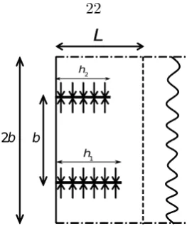
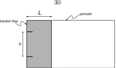
We assume that the arrangement of cracks is periodic, with n cracks in one period. The cracks are equispaced, with spacing b, but have possibly different lengths. For specificity, we specialize to the case of two cracks in one period as shown in Figure 2.4. The semi-infinite strip is subject to periodic boundary conditions on the top and
bottom surfaces, the free edge is traction free, and the crack faces are subject to a normal traction−σ0. As shown in [73], we can write the traction boundary conditions
for the crack faces in terms of dislocation distributionsD1(t) andD2(t) as follows:
π 2b
Z h1
0
D1(t)G1(t, x)dt+
π 2b
Z h2
0
D2(t)G2(t, x)dt=−σo 0< x < h1, (2.3.10a)
π 2b
Z h1
0
D1(t)G2(t, x)dt+
π 2b
Z h2
0
D2(t)G1(t, x)dt=−σo 0< x < h2, (2.3.10b)
whereG1(x, t) and G2(t, x) are as follows
G1(t, x) = 2 coth
π(x+t)
2b −
π(x+ 3t) 2b cosech
2π(x+t)
2b +
xtπ2
b2 cosech
2π(x+t)
2b coth
π(x+t) 2b −2 cothπ(x−t)
2b +
π(x−t)2
2b cosech
2π(x−t)
2b , (2.3.11a)
G2(t, x) = 2 tanh
π(x+t)
2b +
π(x+ 3t) 2b sech
2π(x+t)
2b −
π2tx
b2 sech
2π(x+t)
2b tanh
π(y+t) 2b −2 tanhπ(y−t)
2b −
π(x−t) 2b sech
2π(y−t)
2b . (2.3.11b)
2b
1 h
2 h
L
b
Figure 2.4: Unit cell of width 2bcontaining two cracks, chosen for the analysis
singularity we rewrite D1 and D2 as
D1(t) =
h1
p
h2 1−t2
C1(t), D2(t) =
h2
p
h2 2−t2
C2(t). (2.3.12)
The integral equations are solved numerically by using Gauss-Chebyshev quadrature forC1 and C2. The Mode-I stress intensity factors can be expressed as
Ki = lim x→h+i
p
2π(x−hi)σyy(x, y= 0) =−π
p
πhiCi(hi) i= 1,2. (2.3.13)
See AppendixA.2for further details. The values obtained were verified against those listed in literature [14].
Note that the cracks are subjected to stresses that are analogous to Mode-I loading – i.e., the stresses seek to open the crack. In this situation, the driving force da on the
crack is related to the stress intensity factor defined in (2.3.13) as [86] :
dia= K
2
i
E . (2.3.14)
2.4
Phase boundary
−4 −3.5 −3 −2.5 −2 −1.5 −1 −0.5 0 0.5−0.5 −0.4 −0.3 −0.2 −0.1 0 0.1 0.2 0.3 0.4
dcrack/σoεo
y/b
L/b = 1.6 L/b = 1.55 L/b = 1.52
(a)
−0.2 −0.15 −0.1 −0.05 0 0.05 0.1 0.15−0.5 −0.4 −0.3 −0.2 −0.1 0 0.1 0.2 0.3 0.4 0.5 f/b y/b L/b = 1.6
L/b = 1.55 L/b = 1.52
(b)
Figure 2.5: (a) Normalized driving force on the phase boundary due to the presence of the cracks over one unit cell containing a single crack. Negative values indicate force towards the cracks. The mean value over one unit cell is zero. (b) The equilibrium shape of the phase boundary. In both figures, we use b = 10mm, h = h1 = h2 = 15mm, L =
15.2mm,15.5mm,16mm.
cracks. So we consider a unit cell containing a single crack.
We begin by examining the driving force acting on the phase boundary. This is given by (2.2.13). In light of the superposition described in Section 2.3.2, this driving force may be decomposed as
dS=d0+dself+dcrack, (2.4.1)
where
d0 = hσAi:ε?−ω
, dself=hσBi:ε?, dcrack=σC :ε?. (2.4.2)
The first term is the driving force on a planar phase boundary in the absence of cracks. The second term is the driving force resulting from the non-planar nature of the phase boundary. The third is the driving forces due to the presence of cracks, and specifically due to the stress resulting from the sub-problem C. Further, since ε∗ is of the form (2.3.7),
dcrack=−ε0(2σ11(C)+σ (C)
22 ). (2.4.3)
towards the crack ahead of the crack, and pushed away from it between two cracks. This is as we expect from intuition given that theβ phase is longer in they direction compared to the α phase. We also find numerically that the mean value of this contribution to the driving force over the entire unit cell is zero. We expect from the equilibrium of the unit cell (Figure2.4) that average value ofσ(11C) to be zero. We find numerically that the average of σ22(C) also turns out the to be zero.
We now turn to propagation. The driving force created by the cracks tends to distort the phase boundary away from the planar shape. This leads to self-interaction which in turn depends on the shape of the phase boundary. To understand this, we study the equilibrium shape of the phase boundary under the assumption that there is no driving force on the planar boundary. In other words, we solve the equation dself+dcrack = 0 for the normal
distortion x = f(y). A typical result is shown in Figure 2.5 (b). The driving force due to sub-problem (C) tends to distort the phase boundary while the self-energy tends to straighten it out. The overall result is a phase boundary drawn towards the crack ahead of the crack, and pushed away from it between two cracks, with mean distortion zero. Now, for an interface with this shape, dS = d0. Since d0 is independent of shape, the driving
force is uniform and according to (2.2.16), the interface propagates as long as the chemical driving force is large without any further distortion and subject to the same driving force as a straight interface.
In summary, while the cracks may potentially distort the phase boundary locally, it does not affect the overall evolution. Combined with the earlier observation that the stresses due to the distorted phase boundary decay away from it, we assume henceforth that the phase boundary propagates independent of the cracks and the cracks only see a planar phase boundary.
2.5
Crack propagation
2.5.1 Cracks with uniform spacing and length
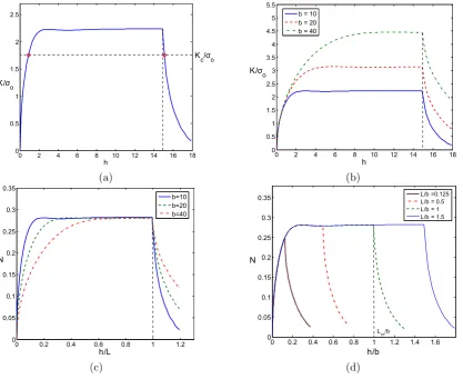
0 2 4 6 8 10 12 14 16 18 0 0.5 1 1.5 2 2.5 h K/σo
Kc/σo
(a)
0 2 4 6 8 10 12 14 16 18
0 0.5 1 1.5 2 2.5 3 3.5 4 4.5 5 5.5 h K/σo
b = 10 b = 20 b = 40
(b)
0 0.2 0.4 0.6 0.8 1 1.2
0 0.05 0.1 0.15 0.2 0.25 0.3 0.35 h/L N b=10 b=20 b=40 (c)
0 0.2 0.4 0.6 0.8 1 1.2 1.4 1.6 0 0.05 0.1 0.15 0.2 0.25 0.3 0.35 h/b N L/b =0.125 L/b = 0.5 L/b = 1 L/b = 1.5
Lcr/b
(d)
and examine the driving force or equivalently the stress intensity experienced by the crack. Figure2.6(a) shows the stress intensity factor (normalized by nominal stress) as a function of crack-length for a given spacing. As anticipated, the stress intensity vanishes at zero crack length and gradually increases with crack length. The variation is similar to that of an isolated edge crack. As the crack length increases, the cracks begin to interact with each other and shield each other. So, the rate of increase of stress intensity with length decreases; eventually it peaks (at h= 2.9mm withK/σ0 = 2.229√mmfor b= 10mm). It
drops slightly beyond the peak but then increases slightly again to reach a limiting value independent of crack-length (K∞/σ0 = 2.236√mm for b = 10mm). We label this the
limiting stress intensity K∞. We understand this limit as follows: once the cracks become
long and no longer feel the presence of the free edge, they behave like a system of parallel semi-infinite cracks. The situation changes when the crack reaches the phase boundary. It drops rapidly as the state of stress changes on the other side of the phase boundary.
Figure2.6(b) shows the stress intensity for various crack-spacing. We see that the stress intensity factor increases with increasing spacing due to reduced interaction (shielding) between the cracks. Figure 2.6(c) shows the same results in a non-dimensional fashion: N = K
σo √
2πb vs. h/L. Remarkably, note that the limiting value of the non-dimensional
stress-intensity, N∞ = 0.282, is independent of the crack spacing. Finally, Figure 2.6(d)
shows that the (non-dimensionalized) stress-intensity vs. crack length is unaffected by the position of the phase boundary, except that it determines the point beyond which the stress intensity drops. We define the position of the phase boundary where the normalized stress intensity factor first reaches the peak valueN∞ to beLcr. It occurs atLcr=b.
Now consider a material with a fracture toughness of Kc. Our crack propagation
crite-rion (2.2.15) is equivalent to the statement that cracks propagate whenK =Kc. If we know
the crack spacing and it is small enough, Figure 2.6(a) shows that there are two possible crack-lengths – one close to the free surface, and one slightly beyond the phase boundary∗. The stability criterion (2.2.19) adopted to a single crack states that the stability is
equiva-∗
lent to requiring that the stress-intensity factor decreases with increasing crack-length (also [73]). Thus, the stable crack position is the one slightly beyond the phase boundary. Since the limiting stress intensity factor is independent of crack length and phase boundary posi-tion, we obtain a simple criterion for crack propagation with a fixed spacing: parallel cracks propagate uniformly when K∞=Kcor equivalentlyN∞=Nc where
Nc=
Kc
σ0
√
2πb?. (2.5.1)
In other words, thecritical transformation strainε?
0 for cracks to propagate with the phase
boundary at spacing bis
ε?0 =
r
6.28 K
2
c
πE2b, (2.5.2)
for cracks to propagate with the phase boundary at spacing b.
The previous discussion assumed a knowledge of the crack spacing. To determine this, we turn to Figure 2.6(b). Notice that the stress intensity increases with increasing crack spacing. Thus, we conclude that the critical crack spacing b? would be the one where the
peak stress intensity is exactly equal to the toughness. Since the peak is close to the limiting value, and since the normalized value of the peak stress intensity factorN∞ is independent
of b, we use the limiting value instead. So we setN∞=Nc. We conclude that theoptimal
crack spacingb? for a material with transformation strainε
0 is
b? = 1
2π K2
c
σ2 0N∞2
= 6.28 K
2
c
πE2ε2 0
. (2.5.3)
Importantly, since thisN∞is independent of phase boundary position (Figure2.6(d)), this
optimal spacing remains unchanged as the phase boundary continues to propagate. Finally, since the stress-intensity falls off beyond the phase boundary independent of the phase boundary position, the stability of a crack with a tip extending just beyond the boundary remains unchanged.
In summary, the previous discussion suggests that the cracks nucleate when the phase boundary propagates to a distance Lcr from the free edge. Then uniformly spaced cracks
with spacing b? nucleate with initial length slightly larger than L
1.4 1.42 1.44 1.46 1.48 1.5 1.52 1.54 1.56 1.58 1.6 0.1
0.12 0.14 0.16 0.18 0.2 0.22 0.24 0.26 0.28
h2/b N
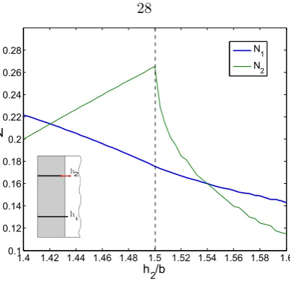
N1 N2
Figure 2.7: Variation of the normalized stress intensity factors (N =K/σ0
√
2πb) experi-enced by the two cracks when the length of one is varied while the that of the other is held fixed. Here, the phase boundary position isL= 15mmindicated by the dotted vertical line while the crack spacing is b= 10mm. Crack #1 has a length h1 = 15.4mmwhile crack #
2 varies in the range [14mm,16mm].
crack propagate with the propagating phase boundary in such a manner that the tips reach just beyond the phase boundary.
2.5.2 Stability against period doubling
It is known that in thermal cracks, there is period doubling instability wherein every al-ternate crack arrests after propagating a certain distance [12,73]. So we study a periodic array of cracks of alternating lengths. We specifically focus on the onset of an instability where both set of cracks have grown equally in a stable fashion as described above, and then one set continues to grow and the other stops. We therefore study the situation where we have a periodic array of equally spaced cracks with alternating lengths.
Figure 2.7shows how the normalized stress intensity factors (Ni =Ki/σ0
√
2πb) experi-enced by the two cracks varies when the length of one crack is varied while that of the other is held fixed (see inset). Specifically, the length of the first crack is held fixed at a position slightly beyond the phase boundary representing the equilibrium crack length (N1 = Nc).
set increases with crack length till it reaches the phase boundary, and subsequently falls. The crack propagation criterion dictates that N1 = N2 = Nc. We see from Figure 2.7
that N1 = N2 for two possible sets of crack-lengths. The first is when the second set of
cracks trails the phase boundary, and the second when the two sets of crack have equal length (just beyond the phase boundary). Since N1 =N2 > Nc for the first case, we focus
on the second whereN1 =N2 =Nc.
To determine the stability, we combine the definition of the Hessian (2.2.20) with the relation between the driving force and stress-intensity factor (2.3.14) to conclude that
Hij = 2
Ki
E ∂Ki
∂hj
. (2.5.4)
We are interested in the situation where one crack continues to propagate while the other crack arrests. In this situation, the sufficient condition for linear stability (i.e., the negation of (2.2.19)) is
∂K1
∂h2
<0, ∂K2 ∂h2
<0. (2.5.5)
(also see [11]). We see in Figure 2.7 that these conditions indeed hold. We have verified that these results hold for various phase boundary positions ranging fromL= 1.5mmwhere we see nucleation to L = 30mm at which point the results converge to that of an infinite system.
We conclude that there is no period doubling instability in phase-transformation driven crack growth.
2.6
Numerical study
The theory above considered only one or two cracks in a unit cell. Further, the stability analysis was limited to linear stability. We use numerical simulations to study multiple cracks in a unit cell and the evolution problem beyond linear stability. After a brief de-scription, we verify the method by showing that the numerical results are consistent with the analysis above and then use it to study more complex situations.
L
b
periodic
traction free
Figure 2.8: Unitcell geometry and boundary conditions.
ABAQUS [1]. We consider plane stress, and a domain that is a long strip. We apply periodic boundary conditions on top and bottom, traction-free conditions on the left and zero displacement on the right, see Figure2.8. Phase transformation is simulated by treating the material as thermo-elastic, and imposing a temperature difference ∆T across a vertical interface representing the phase boundary.
T(x)−T0 =
∆T x≤L
0 x > L
(2.6.1)
The transformation strain is ε0 = α∆T, where α is the coefficient of linear expansion.
We consider both stationary phase boundaries (L = constant) as well as moving phase boundaries (L=L(t)). In the latter we ensure that ˙Lis small enough to ensure quasi-static crack growth.
We use cohesive elements to simulate brittle fracture [17]. We introduce pre-existing cracks or flaws with initial length h0 = 0.1b at the free edge at a spacing b, and place
a series of cohesive elements along the planes ahead of them. This is reasonable because we anticipate only Mode-I cracks to propagate into the solid along horizontal planes. We also note that by introducing flaws, we do not consider nucleation. However, by providing sufficient number of flaws, we let the system choose the crack spacing since not every flaw will develop into a crack. Certain flaws may not develop into cracks, or certain cracks may stop growing thus increasing the spacing between growing cracks.
The material properties we use are as follows : isotropic Young’s modulus E = 410 GPa, Poisson ratioν = 0.14,α= 4×10⁻⁵K−1, fracture toughnessK
c= 4.6M P a√m and
Figure 2.9: Traction-separation law with linear damage evolution.
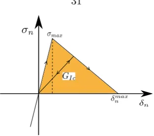
quad elements (CPS4R) were used to discretize the bulk. Four noded, two dimensional Cohesive elements (COH2D4) were used to simulate crack propagation. The constitutive behaviour of the Cohesive elements is governed through a traction-separation law [1]. We present the important details here and describe the choice of parameters for this simulation. The traction-separation law is governed by two regimes. It consists of a linear regime cor-responding to the elastic response of the material prior to initiation of damage. The second regime is the damage response - starting with the onset of damage, evolution of damage and finally suppression of the element - corresponding to deterioration of the material and finally fracture. The damage-onset is based on a criterion which could be traction or displacement based. For this simulation we choose a traction based criterion - damage is initiated once the traction exceeds a peak value. Upon initiation of damage, further loading of the element leads to evolution of the damage captured by a damage evolution law which is represented by the softening portion of the traction-separation law. It must be noted that unloading or compression does not lead to evolution of damage. Various models are available for damage evolution based on effective displacement (to account for mixed-mode loading) or energy. In this case we choose a linear damage evolution law based on effective displacement, see Figure 2.9. The crack is assumed to propagate whenever a cohesive element gets deacti-vated. This happens when the damage parameter attains a value 1.0 at all the material points in the cohesive element. The parameters of initial stiffness and maximum stress of the cohesive element law were chosen based on the criteria described in [111].
0 0.2 0.4 0.6 0.8 1 1.2 1.4 1.6 0
0.05 0.1 0.15 0.2 0.25 0.3 0.35 0.4
h/b N
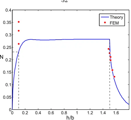
Theory FEM
Figure 2.10: Comparison between predictions of theory and numerical simulation. The red points represent the normalized critical stress intensityNcand final crack length for various
transformation strains computed numerically. The blue curve shows the normalized stress intensity as a function of normalized crack length. Note that cracks do not grow when Nc > N∞ and grow to the phase boundary when N < N∞ showing consistence between
theory and numerical simulation. (b = 0.1mm, L = 0.15mm). The cross-hair on the left indicates the initial flaw.
the stresses and thereby capture crack propagation accurately (see [111] and references therein). Next, the step size for phase boundary propagation should be chosen to resolve the variation of stress intensity factor seen in Figure2.6(a). It was observed during simulations that too big a step size results in artefacts. The convergence difficulties which arise due to the softening behaviour of the cohesive elements are addressed by incorporating viscous regularization [1] and a sufficiently small increment size in the non-linear analysis.
2.7
Results
2.7.1 One flaw in a unit cell
2.7.1.1 Stationary phase boundary
A
C
B
A
B
C
0 0.5 1 1.5 2 2.5 3
0 0.5 1 1.5 2 2.5 3 3.5
L/b h/b
0.16 0.20 0.24
Figure 2.11: Crack growth with a moving phase boundary. Left: The crack length as a function of the phase boundary position for three different values of transformation strain (or equivalently ∆T). Right: Three snap-shots forεo= 0.24%. (b= 0.1mm).
the computed normalized crack length for various normalized critical stress intensityNc=
Kc/Eε0
√
2πb. Note that for small transformation strain or large normalized critical stress intensity, the flaw does not develop into a crack. However, above a given transformation strain (or below a given normalized critical stress intensity), the flaw develops into a crack and grows close to the phase boundary.
Figure 2.10 also shows the normalized stress intensity as a function of the normalized crack length computed using the theoretical analysis of the previous section. Notice that the transition from no crack growth to crack growth is consistent with the theoretical criterion Nc = N∞. The small discrepancy in transition is due to the following. We used a
pre-existing crack of a certain length that happened to be smaller than Lcr; so the cracks
propagated when Nc reached the value at the flaw instead of the limiting value. We get
perfect agreement when we use Nf law instead ofN∞ (see Figure 2.10). Further, in these
situations the cracks grow till a position just beyond the phase boundary, again as predicted by the theoretical considerations earlier.
2.7.1.2 Moving phase boundary
(b)
(a) (c)
Figure 2.12: Crack growth with two cracks in a unit cell for varying transformation strains. (a) Three snap-shots with transformation strain of 0.16% shows neither crack grows. (b) Three snap-shots with transformation strain of 0.184% shows the one crack grows along with the phase boundary. (c) Three snap-shots with transformation strain of 0.22% shows the both cracks grow along the grows along with the phase boundary. The flaw spacing is b = 0.1mm and the critical flaw spacing for crack growth at the applied strain based on Nf law are: (a)∞ (b) 0.17mmand (c) 0.056mm.
of transformation strain (or equivalently ∆T). We see that the crack does not grow for the smallest transformation strain, but does for the larger transformation strains. Note that this is consistent with the theory which predicts that for the givenb, the transformation strain has to exceed the critical value ofεo= 0.16% that corresponds to ∆T of 40. Further, when
this happens, the crack trip propagates close to the phase boundary, again as anticipated by the theory presented earlier.
2.7.2 Multiple flaws in a unit cell
0 0.2 0.4 0.6 0.8 1 1.2 1.4 1.6 0 0.2 0.4 0.6 0.8 1 1.2 1.4 L/b h /b crack 1 crack 2 crack 3 crack 4
0 0.2 0.4 0.6 0.8 1 1.2 1.4 1.6 0 0.2 0.4 0.6 0.8 1 1.2 1.4 L/b h /b crack 1 crack 2 crack 3 crack 4
(a) (b) (c)
0 0.2 0.4 0.6 0.8 1 1.2 1.4 1.6 0 0.2 0.4 0.6 0.8 1 1.2 1.4 L/b h/b crack 1 crack 2 crack 3 crack 4
Figure 2.13: Crack growth with four cracks in a unit cell at various transformation strains. Crack length vs interface position for (a)εo= 0.16% (b)εo= 0.184% (c)εo = 0.22%. The
flaw spacing is b= 0.1mm.
and 2b(0.17mm) and (c) smaller thanb(0.056mm). Thus, the theory predicts that with an imposed spacing of two cracks, we should see neither crack growing in case (a), only one of the two cracks growing in case (b) and both cracks growing in case (c). These predictions are indeed confirmed by the results of numerical simulations shown in Figure 2.12. These results also confirm the absence of period doubling instability which was concluded earlier from the linear stability analysis.
Figure 2.13 shows the results of simulations with the unit cell containing four initial flaws. The figure shows the position of each of the flaw tips with phase boundary position at three transformation strains. Through this we can examine the stability of the system to modes other than period doubling mode. The flaw spacing provided is b= 0.1mm. The results show that though the flaws start propagating initially, some of them stop growing and result in attaining the uniform spacing predicted by theory ( see (2.5.3) ) at that strain. One might argue that since half of the cracks stopped propagating in case (b) (Figure2.13) we see a period doubling instability. However this is not the case - this is only the transient response during which a certain spacing between the cracks is established according to (2.5.3). Once uniform spacing is attained, the cracks continue to propagate without any instabilities. If indeed the system were susceptible to period doubling one would have seen one of the two propagating cracks stop at some stage which is not the case. Similarly in case (c), since the transformation strain is high enough and the optimal value of spacing (b∗) given by (2.5.3) is lower than the minimum allowed spacing (b) in the simulation, it is
evidence of instabilities.
2.8
Conclusions
Phase transformations lie at the heart of a number of important technological applications. In these situations the stresses built up due to change in shape resulting from the transfor-mation could cause cracking of the material resulting in compromising the performance of the system. In the current study we seek to understand the interaction between a phase boundary and the cracks resulting due to the phase transition. First we established a con-dition on the jump in stress across a coherent phase boundary due to a phase transition which gives rise to a set of parallel cracks. Next assuming uniform elastic properties we examine the growth of set of edge cracks in the wake of such a propagating phase boundary in two dimensions. We study the effect of cracks on the phase boundary and conclude that they only have the effect of distorting the phase boundary. They do not effect its overall propagation. We examined the equilibrium configurations of cracks and performed a sta-bility analysis to understand their growth pattern. We found that cracks which nucleate at the edge grow all the way to the phase boundary with the crack tips crossing over, and continue to grow in a stable fashion as the phase boundary migrates into the interior. The mode of growth is devoid of any instabilities typically seen in other scenarios like thermal cracking or due to gradients in concentration of species like drying of paint layers and mud-flats. The spacing between these cracks depends on the initial flaw distribution and the strain mismatch of the transformation with the spacing decreasing for higher values of the strain mismatch. These predictions from theory are backed by computational simulations which show that once even spacing between cracks is established they continue to progress without any further instabilities.
2.9
Future Directions
Chapter 3
Effect of Space Charges on
Fracture in Ferroelectric Peroskites
3.1
Introduction
Ferroelectric perovskites are materials with a rich array of interesting properties. These materials attain a spontaneous polarization below their Curie temperature which can be switched through the application of electromechanical fields. In their polarized state they display the piezoelectric property and have high dielectric constants. Also, their opti-cal properties are coupled to their polarization state. As a result these materials have found widespread application in transducing devices, dielectric capacitors, memory and optoelectronic devices. From a mechanical property standpoint commonly used ferroelec-tric perovskites like BaTiO3, PZT are brittle in nature with low fracture toughness values
(KIC ∼1M P a√m). In many of these applications these materials are designed to be used
in multilayer arrangements. The electrodes embedded in the materials serve as sites for crack initiation during the poling process. The resulting cracks show sub-cyclic growth un-der applied electromechanical fields. A prominent issue is the growth of cracks connecting the electrode layers resulting in electric discharge and breakdown, Figure 3.1. This has motivated an effort to understand the fracture behaviour of ferrolectrics.
(a)
(b)
Figure 3.1: Cracks in piezoelectric actuators. (a) Multilayer actuator (b) Electric discharge
materials consistently produced longer cracks normal to the poling direction than those par-allel to it at a given indentation load. Sub-critical crack growth under cyclic electric fields and crack growth under static electric fields in the absence of any applied mechanical load motivated research to establish the dependence of crack growth on the applied electric field. However the experiments undertaken to establish this did not produce consistent trends. The experiments by Mehta and Virkar[69] and Fang et.al [50] established that polarization domain switching around the crack played a significant role in crack growth un
![Figure 1.1: Cubic to monoclinic transformation of Nitinol. Reproduced from [64]](https://thumb-us.123doks.com/thumbv2/123dok_us/1121915.1141262/16.595.226.426.71.189/figure-cubic-monoclinic-transformation-nitinol-reproduced.webp)
![Figure 1.2: Cracks resulting from phase transformation. (a) SEM micrographs of polishedsurfaces of CsHsubjecting to cyclic electric loading [partially delithiated LiFePO2PO4 above the phase transition temperature [65]](https://thumb-us.123doks.com/thumbv2/123dok_us/1121915.1141262/18.595.208.440.52.265/transformation-micrographs-polishedsurfaces-cshsubjecting-partially-delithiated-transition-temperature.webp)