Hae-Jong Seo
and Peyman Milanfar
Abstract
A practical problem addressed recently in computational photography is that of producing a good picture of a poorly lit scene. The consensus approach for solving this problem involves capturing two images and merging them. In particular, using a flash produces one (typically high signal-to-noise ratio [SNR]) image and turning off the flash produces a second (typically low SNR) image. In this article, we present a novel approach for merging two such images. Our method is a generalization of the guided filter approach of He et al., significantly improving its performance. In particular, we analyze the spectral behavior of the guided filter kernel using a matrix formulation, and introduce a novel iterative application of the guided filter. These iterations consist of two parts: a nonlinear anisotropic diffusion of the noisier image, and a nonlinear reaction-diffusion (residual) iteration of the less noisy one. The results of these two processes are combined in an unsupervised manner. We demonstrate that the proposed approach outperforms state-of-the-art methods for both flash/no-flash denoising, and deblurring.
1 Introduction
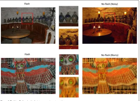
Recently, several techniques [1-5] to enhance the quality of flash/no-flash image pairs have been proposed. While the flash image is better exposed, the lighting is not soft, and generally results in specularities and unnatural appearance. Meanwhile, the no-flash image tends to have a relatively low signal-to-noise ratio (SNR) while contain-ing the natural ambient lightcontain-ing of the scene. The key idea of flash/no-flash photography is to create a new image that is closest to the look of the real scene by hav-ing details of the flash image while maintainhav-ing the ambi-ent illumination of the no-flash image. Eisemann and Durand [3] used bilateral filtering [6] to give the flash image the ambient tones from the no-flash image. On the other hand, Petschnigg et al. [2] focused on reducing noise in the no-flash image and transferring details from the flash image to the no-flash image by applying joint (or cross) bilateral filtering [3]. Agrawal et al. [4] removed flash artifacts, but did not test their method on no-flash images containing severe noise. As opposed to a visible flash used by [2-4], recently Krishnan and Fergus [7] used both near-infrared and near-ultraviolet illumination
for low light image enhancement. Their so-called“dark
flash”provides high-frequency detail in a less intrusive
way than a visible flash does even though it results in incomplete color information. All these methods ignored any motion blur by either depending on a tripod setting or choosing sufficiently fast shutter speed. However, in practice, the captured images under low-light conditions using a hand-held camera often suffer from motion blur caused by camera shake.
More recently, Zhuo et al. [5] proposed a flash deblur-ring method that recovers a sharp image by combining a blurry image and a corresponding flash image. They integrated a so-called flash gradient into a maximum-a-posteriori framework and solved the optimization pro-blem by alternating between blur kernel estimation and sharp image reconstruction. This method outperformed many states-of-the-art single image deblurring [8-10] and color transfer methods [11]. However, the final out-put of this method looks somewhat blurry because the model only deals with a spatially invariant motion blur.
Others have used multiple pictures of a scene taken at different exposures to generate high dynamic range images. This is called multi-exposure image fusion [12] which shares some similarity with our problem in that it seeks a new image that is of better quality than any of the input images. However, the flash/no-flash photography is generally more difficult due to the fact that there are only a pair of images. Enhancing a low SNR no-flash image
* Correspondence: [email protected] 1Sharp Labs of America, Camas, WA 98683, USA
Full list of author information is available at the end of the article
with a spatially variant motion blur only with the help of a single flash image is still a challenging open problem.
2 Overview of the proposed approach
We address the problem of generating a high quality
image from two captured images: a flash image (Z ) and
a no-flash image (Y ; Figure 1). We treat these two
images,Zand Y, as random variables. The task at hand
is to generate a new image (X) that contains the
ambi-ent lighting of the no-flash image (Y) and preserves the
details of the flash-image (Z). As in [2], the new image
Xcan be decomposed into two layers: a base layer and a
detail layer;
X=Y
base
+τ(Z−Z)
det ail .
(1)
Here,Ymight be noisy or blurry (possibly both), and
Y is an estimated version ofY, enhanced with the help
of Z. Meanwhile,Z represents a nonlinear, (low-pass)
filtered version of Zso that Z−Z can provide details.
Note thatτ is a constant that strikes a balance between
the two parts. In order to estimateY andZ, we employ
local linear minimum mean square error (LMMSE)
pre-dictorsawhich explain, justify, and generalize the idea of
guided filteringbas proposed in [1]. More specifically,
we assumed thatY andZare a liner (affine) function of
Zin a windowωkcentered at the pixelk:
yi=G(yi,zi) =azi+b,
zi=G(zi,zi) =czi+d,∀i∈ωk,
(2)
whereG(·) is the guided filtering (LMMSE) operator,
zi, zi, zi are samples of Y, Z,Z respectively, at pixeli,
and (a, b,c, d) are coefficients assumed to be constant
inωk(a square window of sizep×p) and space-variant.
Once we estimatea,b,c,d, Equation 1 can be rewritten
as
xi=yi+τ(zi−zi),
=azi+b+τzi−τczi−τd, = (a−τc+τ)zi+b−τd, =αzi+β.
(3)
In fact,xˆiis a linear function ofzi. While it is not
pos-sible to estimate aand bdirectly from (equation (3);
ˆ
xi,n=G(xˆi,n−1,zi) +τn(zi− ˆzi) =αnzi+βn, (4)
wherexˆi,0=yiandan, bn, andτn are functions of the
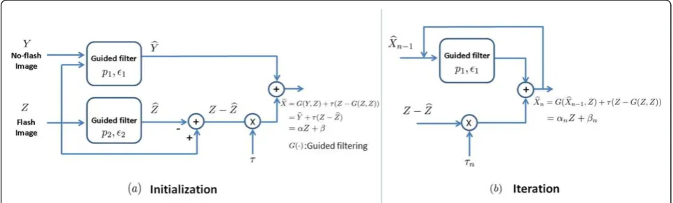
iteration number n. A block-diagram of our approach is
shown in Figure 2. The proposed method effectively removes noise and deals well with spatially variant motion blur without the need to estimate any blur ker-nel or to accurately register flash/no-flash image pairs when there is a modest displacement between them.
A preliminary version [13] of this article is appeared in the IEEE International Conference on Computer
Vision (ICCV ‘11) workshop. This article is different
from [13] in the following respects:
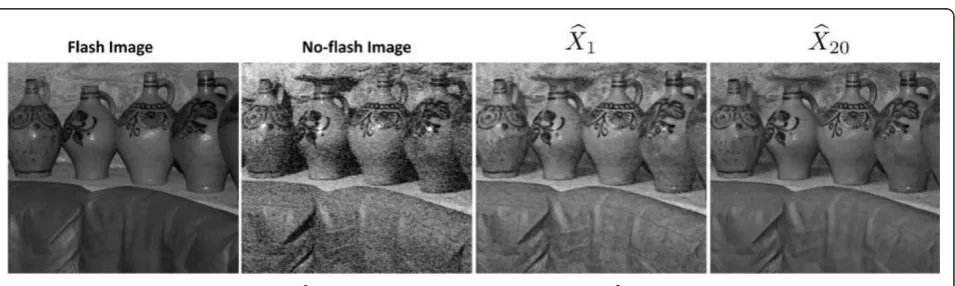
(1) We have provided a significantly expanded statis-tical derivation and description of the guided filter and its properties in Section 3 and Appendix. (2) Figures 3 and 4 are provided to support the key idea of iterative guided filtering.
(3) We provide many more experimental results for both flash/no-flash denoising and de- blurring in Section 5.
(4) We describe the key ideas of diffusion and resi-dual iteration and their novel relevance to iterative guided filtering in the Appendix.
(5) We prove the convergence of the proposed itera-tive estimator in the Appendix.
(6) As supplemental material, we share our project
websitec
where flash/no-flash relighting examples are also presented.
3 The guided filter and its properties
In general, space-variant, nonparametric filters such as the bilateral filter [6], nonlocal means filter [14], and locally adaptive regression kernels filter [15] are esti-mated from the given corrupted input image to perform denoising. The guided filter can be distinguished from these in the sense that the filter kernel weights are com-puted from a (second) guide image which is presumably cleaner. In other words, the idea is to apply filter kernels
Wijcomputed from the guide (e.g., flash) imageZto the
more noisy (e.g., no-flash) imageY. Specifically, the filter
output sample y a pixeli is computed as a weighted
averaged:
ˆ
yi=
j
Wij(Z)yj. (5)
Note that the filter kernel Wij is a function of the
guide imageZ, but is independent ofY. The guided
fil-ter kernelecan be explicitly written as
Wij(Z) = 1 |ω|2
k:(i,j)∈ωk
1 +(zi−E[Z]k)(zj−E[Z]k) var(Z)k+ε
, i,j∈ωk, (6)
where |ω| is the total number of pixels (=p2) inωk,ε
is a global smoothing parameter, E[Z]k≈ |ω1|l∈ωkzl,
and var(Z)k≈ |ω1|
l∈ωk
z2l −E[Z]2k. Note that W
ij are
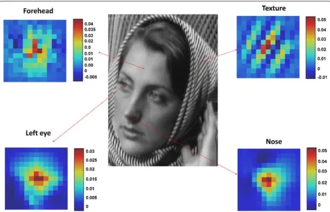
nor-malized weights, that is, ∑jWij(Z) = 1 Figure 5 shows
examples of guided filter weights in four different
patches. We can see that the guided filter kernel weights neatly capture underlying geometric structures as do other data-adaptive kernel weights [6,14,15]. It is worth noting that the use of the specific form of the guided fil-ter here may not be critical in the sense that any other
data-adaptive kernel weights such as non-local means
kernels[16] and locally adaptive regression kernels[15] could be used.
Next, we study some fundamental properties of the guided filter kernel in matrix form.
We adopt a convenient vector form of Equation 5 as follows:
ˆ
yi=wTiy, (7)
where y is a column vector of pixels in Y and
wT
i = [W(i, 1),W(i, 2),. . .,W(i,N)] is a vector of
weights for each i. Note that Nis the dimensionf ofy.
Writing the above at once for alliwe have,
y = ⎡ ⎢ ⎢ ⎢ ⎣
wT
1 wT
2 .. .
wT N
⎤ ⎥ ⎥ ⎥ ⎦=
⎡ ⎢ ⎢ ⎢ ⎣
W(1, 1) W(1, 2). . . W(1,N)
W(2, 1) W(2, 2). . . W(2,N) ..
. ... . .. ...
W(N, 1)W(N, 2). . .W(N,N) ⎤ ⎥ ⎥ ⎥
⎦=W(z)y, (8)
where z is a vector of pixels in Z and W is only a
function ofz. The filter output can be analyzed as the
product of a matrix of weightsWwith the vector of the
given the input imagey.
Figure 3Iteration improves accuracy. Accuracy of(αˆ20,βˆ20)is improved upon(αˆ1,βˆ1).
Figure 4Effect of iteration. As opposed toX
The matrix W is symmetric as shown in Equation 8
and the sum of each row ofW is equal to one (W1N=
1N) by definition. However, as seen in Equation 6, the
definition of the weights does not necessarily imply that
the elements of the matrix W are positive in general.
While this is not necessarily a problem in practice, we find it useful for our purposes to approximate this ker-nel with a proper admissible kerker-nel [17]. That is, for the
purposes of analysis, we approximateW as a positive
valued, symmetric positive definite matrix with rows summing to one, as similarly done in [18]. For the details, we refer the reader to the Appendix A.
With this technical approximation in place, all
eigen-valuesli(i= 1, ..., N) are real, and the largest eigenvalue
ofW is exactly one (l1 = 1), with corresponding
eigen-vector v1= (1/
√
N)[1, 1,. . ., 1]T= (1/√N)1N as shown
in Figure 6. Intuitively, this means that filtering by W
will leave a constant signal (i.e., a “flat” image)
unchanged. In fact, with the rest of its spectrum inside
the unit disk, powers ofWconverge to a matrix of rank
one, with identical rows, which (still) sum to one:
lim n→∞W
n=1
NuT1. (9)
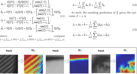
So u1 summarizes the asymptotic effect of applying
the filterWmany times. Figure 7 shows what a typical
u1looks like.
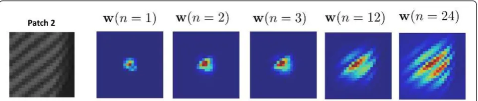
Figure 8 shows examples of the (center) row vector
(wT) from W’s powers in one patch of size 25 × 25. The
vector was reshaped into an image for illustration
pur-poses. We can see that powers ofW provide even better
structure by generating larger (and more sophisticated)
kernels. This insight reveals that applying W multiple
times can improve the guided filtering performance, which leads us to the iterative use of the guided filter.
This approach will produce the evolving coefficientsan,
bn introduced in (4). In the following section, we
describe how we actually compute these coefficients based on Bayesian mean square error (MSE) predictions.
4 Iterative application of local LMMSE predictors
The coefficientsg ak, bk,ck,dkin (3) are chosen so that
“on average” the estimated value Y is close to the
observed value ofY(=yi) inωk, and the estimated value
Z is close to the observed value ofZ(=zi) in ωk. More
specifically, we adopt a stabilized MSE criterion in the
windowωkas our measure of closenessh:
MSE(ak,bk) =E[(Y−Y)2] +ε1ak2=E[(Y−akZ−bk)2] +ε1a2k, MSE(ck,dk) =E[(Z−Z)2] +ε2ck2=E[(Z−ckZ−dk)2] +ε2c2k,
(10)
whereε1 andε2 are small constants that preventaˆk,cˆk
from being too large. Note thatckanddkbecome simply
1 and 0 by settingε2= 0. By setting partial derivatives of
MSE(ak,bk) with respect toak,bk, and partial derivatives
of MSE(ck, dk) with respect to ck, dk, respectively, to
zero, the solutions to minimum MSE prediction in (10) are
ˆ
ak=
E[ZY]−E[Z]E[Y] E[Z2]−E2[Z] +ε
1 =
cov(Z,Y) var(Z) +ε1
k ,
ˆ
bk=E[Y]− ˆakE[Z] =E[Y]k−
cov(Z,Y) var(Z) +ε1
k
E[Z]k,
ˆ
ck=
E[Z2]−E2[Z] E[Z2]−E2[Z] +ε
2 =
var(Z) var(Z) +ε2
k ,
ˆ
dk=E[Z]− ˆckE[Z] =E[Z]k−
var(Z) var(Z) +ε2
k
E[Z]k,
(11)
where we compute
E[Z]≈ 1
|ω|
l∈ωkzl,E[Y]≈
1
|ω|
l∈ωkyl,E[ZY]≈
1
|ω|
l∈ωkzlyl,E[Z
2]≈ 1
|ω|
l∈ωkz
2
l.
Note that the use of different ωk results in different
predictions of these coefficients. Hence, one must com-pute an aggregate estimate of these coefficients coming from all windows that contain the pixel of interest. As
an illustration, consider a case where we predictyi using
observed values of Y in ωk of size 3 × 3 as shown in
Figure 9. There are nine possible windows that involve
the pixel of interesti. Therefore, one takes into account
all nine ak, bk’s to predict yi. The simple strategy
sug-gested by He et al. [1] is to average them as follows:
ˆ
a= 1
|ω|
|ω|
k=1
ˆ
ak,bˆ= 1 |ω| |ω| k=1 ˆ
bk. (12)
As such, the resulting prediction of Y given the
out-comeZ=ziis
ˆ
yi=azˆ i+bˆ= 1
|ω|
|ω|
k=1
(aˆkzi+bˆk),
ˆ
zi=czˆ i+dˆ= 1
|ω|
|ω|
k=1
(ˆckzi+dˆk).
(13)
Figure 6Examples of W in one patch of size 25 × 25. All eigenvalues of the matrixWare nonnegative, thus the guided filter kernel matrix is positive definite matrix. The largest eigenvalue ofWis one and the rank ofWasymptotically becomes one. This figure is better viewed in color.
The idea of using these averaged coefficients aˆ,bˆ is analogous to the simplest form of aggregating multiple local estimates from overlapped patches in image denoising and super-resolution literature [19]. The aggregation helps the filter output look locally smooth
and contain fewer artifacts.i Recall that yi and ˆzi−zi
correspond to the base layer and the detail layer,
respec-tively. The effect of the regularization parametersε1and
ε2 is quite the opposite in each case in the sense that
the higherε2 is, the more detail through ˆzi−zican be
obtained; whereas the lower ε1 ensures that the image
content inY is not over-smoothed.
These local linear models work well when the window
size pis small and the underlying data have a simple
pattern. However, the linear models are too simple to deal effectively with more complicated structures, and thus there is a need to use larger window sizes. As we alluded to earlier, the estimation of these linear coeffi-cients in an iterative fashion can deal well with more complex behavior of the image content. More
Figure 8The guided filter kernel matrix. The guided filter kernel matrixWcaptures the underlying data structure, but powers ofWprovides even better structure by generating larger (but more sophisticated) kernel shapes.wis the (center) row vector ofW.wwas reshaped into an image for illustration purposes.
Figure 9Explanation of LMMSE.aˆk,bˆkare estimated from nine different windowsωkand averaged coefficientsaˆ,bˆare used to
specifically, by initializing ˆxi,0=yi, Equation 3 can be
updated as follows
ˆ
xi,n = G(xˆi,n−1, zi) +τn(zi− ˆzi), = (an−τnc+τn)zi+bn−τnd, =αnzi+βn,
(14)
wherenis the iteration number andτn>0 is set to be a
monotonically decaying functionkofnsuch that∞n=1τn
converges. Figure 3 shows an example to illustrate that the resulting coefficients at the 20th iteration predict the
underlying data better than a1, b1 do. Similarly, X20
improves uponX1as shown in Figure 4. This iteration is
closely related todiffusionandresidual iterationwhich are
two important methods [18] which we describe briefly below, and with more detail in Appendix.
Recall that Equation 14 can also be written in matrix form as done in Section 3:
ˆ
xn= W xˆn−1
base layer
+τn(z −Wdz) det ail layer
,
(15)
where W and Wd are guided filter kernel matrices
composed of the guided filter kernelsWandWd
respec-tively.lExplicitly writing the iterations, we observe
ˆ
x0=y ˆ
x1=Wy+τ1(I−Wd)z, ˆ
x2=Wxˆ1+τ2(I−Wd)z=W2y+ (τ1W+τ2I)(I−Wd)z,
.. .
ˆ
xn=Wxn−ˆ 1+τn(I−Wd)z=Wny+ (τ1Wn−1+τ2Wn−2+· · ·+τnI)(I−Wd)z,
= Wny
diffusion
+Pn(W)(I−Wd)z
residual iteration
=ynˆ +ˆzn,
(16)
wherePnis a polynomial function ofW. The
block-dia-gram in Figure 2 can be redrawn in terms of the matrix
formulation as shown in Figure 10. The first termyˆnin
Equation 16 is called the diffusion process that enhances
SNR. The net effect of each application ofWis
essen-tially a step of anisotropic diffusion [20]. Note that this
diffusion is applied to the no-flash imageywhich has a
low SNR. On the other hand, the second termzˆnis
con-nected with the idea of residual iteration [21]. The key
idea behind this iteration is to filter the residual signalsm
to extract detail. We refer the reader to Appendix B and [18] for more detail. By effectively combining the diffu-sion and residual iteration [as in (16)], we can achieve the goal of flash/no-flash pair enhancement which is to
gen-erate an image somewhere between the flash imagezand
the no-flash imagey, but of better quality than both.n
5 Experimental results
In this section, we apply the proposed approach to flash/ no-flash image pairs for denoising and deblurring. We
convert imagesZand Yfrom RGB color space to CIE
Lab, and perform iterative guided filtering separately in each resulting channel. The final result is converted back to RGB space for display. We used the implementation of
the guided filter [1] from the author’s website.oAll
fig-ures in this section are best viewed in color.p
5.1 Flash/no-flash denoising 5.1.1 Visible flash [2]
We show experimental results on a couple of flash/no-flash image pairs where no-flash/no-flash images suffer from
noiseq. We compare our results with the method based
on the joint bilateral filter [2] in Figures 11, 12, and 13. Our proposed method effectively denoised the no-flash image while transferring the fine detail of the flash image and maintaining the ambient lighting of the no-flash image. We point out that the proposed iterative application of the guided filtering in terms of diffusion and residual iteration yielded much better results than one application of either the joint bilateral filtering [2] or the guided filter [1].
5.1.2 Dark flash [7]
In this section, we use thedark flashmethod proposed
in [7]. Let us call the dark flash image Z. Dark flash
may introduce shadows and specularities in images, which affect the results of both the denoising and detail transfer. We detect those regions using the same meth-ods proposed by [2]. Shadows are detected by finding
the regions where|Z-Y| is small, and specularities are
found by detecting saturated pixels inZ. After
combin-ing the shadow and specularities mask, we blur it uscombin-ing a Gaussian filter to feather the boundaries. By using the
resulting mask, the output Xnat each iteration is
alpha-blended with a low-pass filter version of Yas similarly
done in [2,7]. In order to realize ambient lighting condi-tions, we applied the same mapping function to the final output as in [7]. Figures 14, 15, 16, 17, 18, and 19 show that our results yield better detail with less color arti-facts than the results of [7].
5.2 Flash/no-flash deblurring
Motion blur due to camera shake is an annoying yet com-mon problem in low-light photography. Our proposed
method can also be applied to flash/no-flash deblurringr.
Figure 24 while Zhuo et al. [5] used two blurred images and one flash image.
6 Summary and future work
The guided filter has proved to be more effective than the joint bilateral filter in several applications. Yet we
have shown that it can be improved significantly more still. We analyzed the spectral behavior of the guided fil-ter kernel using a matrix formulation and improved its performance by applying it iteratively. Iterations of the proposed method consist of a combination of diffusion and residual iteration. We demonstrated that the
Figure 10Diagram of the proposed iterative approach in matrix form. Note that the iteration can be divided into two parts: diffusion and residual iteration process.
Figure 12Flash/no-flash denoising example compared to the state of the art method[2]. The iterationnfor this example is 10.
Figure 14Dark flash/no-flash (low noise) denoising example compared to the state of the art method[7]. The iterationnfor this example is 10.
Figure 16Dark flash/no-flash (high noise) denoising example compared to the state of the art method[7]. The iterationnfor this example is 10.
Figure 18Dark flash/no-flash (mid noise) denoising example compared to the state of the art method[7]. The iterationnfor this example is 10.
proposed approach yields outputs that not only preserve fine details of the flash image, but also the ambient lighting of the no-flash image. The proposed method outperforms state-of-the-art methods for flash/no-flash
image denoisinganddeblurring. It would be interesting
to see if the performance of other nonparametric filer kernels such as bilateral filters and locally adaptive regression kernels [15] can be further improved in our iterative framework. It is also worthwhile to explore sev-eral other applications such as joint upsampling [22], image matting [23], mesh smoothing [24,25], and specu-lar highlight removal [26] where the proposed approach can be employed.
Appendix
Positive definite and symmetric row-stochastic approximation of W
In this section, we describe how we approximate W
with a symmetric, positive definite, and row-stochastic
matrix. First, as we mentioned earlier, the matrix W
can contain negative values as shown in Figure 3. We
employ the Taylor series approximation (exp (t) ≈1 +
t) to ensure thatW has both positive elements, and is
positive-definite. To be more concrete, consider a
sim-ple examsim-ple; namely, a local patch of size 5× 5 as
fol-lows:
Z=
⎧ ⎪ ⎪ ⎪ ⎪ ⎨ ⎪ ⎪ ⎪ ⎪ ⎩
z1 z6 z11z16z21
z2 z7 z12z17z22
z3 z8 z13z18z23
z4 z9 z14z19z24
z5z10z15z20z25
⎫ ⎪ ⎪ ⎪ ⎪ ⎬ ⎪ ⎪ ⎪ ⎪ ⎭
(17)
In this case, we can have up to 9 ωkof size |ω| = 3×
3. Let Mzi,zj
=
k:(i,j∈ωk)
zi−E[Z]k zj−E[Z]k
var(Z)k+ε
in
Equation 6. Then, W centered at the index 13 can be
written and approximated as follows:
Figure 21Flash/no-flash deblurring example compared to the state-of-the-art method[5]. The iterationnfor this example is 20.
Figure 23Flash/no-flash deblurring example compared to the state-of-the-art method[5]. The iterationnfor this example is 5.
metric, positive definite matrix as again done in [18]. The algorithm we use to effect this approximation is due to Sinkhorn [27,28], who proved that given a matrix with strictly positive elements, there exist diagonal
matrices R= diag(r) andC= diag(c) such that
W=R W C
is doubly stochastic. That is,
W1N=1Nand1TNW=1TN (18)
Furthermore, the vectorsrandcare unique to within
a scalar (i.e.,ar, c/a.) Sinkhorn’s algorithm for
obtain-ing randcin effect involves repeated normalization of
the rows and columns (see Algorithm 1 for details) so that they sum to one, and is provably convergent and optimal in the cross-entropy sense [29].
Algorithm 1 Algorithm for scaling a matrix A to a
nearby doubly-stochastic matrixAˆ
Given a matrix A, let (N,N) be size(A) and initialize
r= ones(N, 1);
fork= 1 :iter;
c= 1./(ATr);
r= 1./(A c);
end
C= diag(c);R= diag(r);
A=RAC
Diffusion and residual iteration Diffusion
Here, we describe how multiple direct applications of
the filter given by W is in effect equivalent to a
non-linear anisotropicdiffusion process [20,30]. We define
ˆ
y0=y, and
ˆ
yn=Wyˆn−1=Wny. (19)
From the iteration (19) we have
ˆ
yn=Wyˆn−1, (20)
=yˆn−1− ˆyn−1+Wyˆn−1, (21)
=yˆn−1+ (W−I)yˆn−1, (22)
which we can rewrite as
ˆ
yn− ˆyn−1= (W−I)ˆyn−1←→
∂¯y(t) ∂t =∇
2y(t)¯ Diffusion Equation (23)
to consider theresidualsignals, defined as the difference
between the estimated signal and the measured signal. This results in a variation of the diffusion estimator which uses the residuals as an additional forcing term. The net result is a type of reaction-diffusion process [31]. In statistics, the use of the residuals in improving estimates has a rather long history, dating at least back
to the study of Tukey [21] who termed the idea “
twi-cing”. More recently, the idea has been suggested in the
applied mathematics community under the rubric of
Bregman iterations [32], and in the machine learning
and statistics literature [33] asL2-boosting.
Formally, the residuals are defined as the difference between the estimated signal and the measured signal:
rn=z−zn−1, where here we define the initializations
ˆ
z0=Wz. With this definition, we write the iterated
esti-mates as
ˆ
zn=zˆn−1+Wrn=zˆn−1+W(z− ˆzn−1). (24)
Explicitly writing the iterations, we observe:
ˆ
z1 = zˆ0+W(z− ˆz0) =Wz+W(z−Wz) = (2W−W2)z,
ˆ
z2 = zˆ1+W(z− ˆz1) = (W3−3W2+ 3W)z, ..
. ˆ
zn=Fn(W)Z,
(25)
whereFnis a polynomial function of Wof order n+
1. The first iteratezˆ1is precisely the“twicing” estimate
of Tukey [21].
Convergence of the proposed iterative estimator
Recall the iterations:
ˆ
xn=Wny+ (τ1Wn−1+τ2Wn−2+· · ·+τnI)
Pn(W)
(I−Wd)z.
(26)
where Pn is a polynomial function of W. The first
(direct diffusion) term in the iteration is clearly stable and convergent as described in (9). Hence, we need to show the stability of the second part. To do this, we
note that the spectrum of Pn can be written, and
bounded in terms of the eigenvaluesliofWas follows:
λi(Pn) = eig(Pn) =τ1λni−1+τ2λni−2+· · ·+τn,
≤τ1λn1−1+τ2λn1−2+· · ·+τn=τ1+τ2+τ3+· · ·+τn≤c.
where the inequality follows from the knowledge that
0 ≤lN ≤... l3 ≤l2 <l1= 1. Furthermore, in Section 4
we definedτnto be a monotonically decreasing sequence
such that∞n=1τn=c<∞. Hence, all eigenvalues li(Pn)
are upper bounded by the constant c, independent of
the number of iterationsn, ensuring the stability of the
iterative process.
End notes a
More detail is provided in Section 4.bThe guided filter
[1] reduces noise while preserving edges as bilateral fil-ter [6] does. However, the guided filfil-ter outperforms the bilateral filter by avoiding the gradient reversal artifacts that may appear in such applications as detail enhance-ment, high dynamic range (HDR) compression, and
flash/no-flash denoising. chttp://users.soe.ucsc.edu/
~milanfar/research/rokaf/.html/IGF/.d yˆ in Equation 2
can be rewritten in terms of filtering and we refer the reader to a supplemental material http://personal.ie. cuhk.edu.hk/~hkm007/eccv10/eccv10supp.pdf for
deri-vation.eCross (or joint) bilateral filter [2,3] is defined in
a similar way.fNis different from the window sizep(N
≥p).gNote that kis used to clarify that the coefficients
are estimated for the window ωk. h Shan et al. [8]
recently proposed a similar approach for high dynamic
range compression. i It is worthwhile to note that we
can benefit from more adaptive way of combining multi-ple estimates of coefficients, but this subject is not
trea-ted in this article. k We useτn=
1
n2 throughout the all
experiments. lRecall Win Equation 6. The difference
betweenWand Wdlies in the parameterεas follows (ε2
>ε1):
W(Z)= 1
|ω|2
k:(i,j)∈ωk
1 +(zi−E[z]k)
zj−E[Z]k
var(Z)k+ε1
,
Wd(Z)=
1
|ω|2
k:(i,j)∈ωk
1 +(zi−E[z]k)
zj−E[Z]k
var(Z)k+ε2
. (28)
m
This is generally defined as the difference between
the estimated signal Zand the measured signal Z, but
in our context refers to the detail signal. nWe refer the
reader to Appendix C for proof of convergence of the
proposed iterative estimator. ohttp://personal.ie.cuhk.
edu.hk/~hkm007/. pWe refer the reader to the project
Website http://users.soe.ucsc.edu/~milanfar/research/
rokaf/.html/IGF/. qThe window size pfor Wd and W
was set to 21 and 5 respectively for all the denoising
examples. rThe window sizep forWdand W was set
to 41 and 81, respectively, for the deblurring examples to deal with displacement between the flash and
no-flash image.s
Note that due to the use of residuals, this
is a different initialization than the one used in the dif-fusion iterations.
Acknowledgements
We thank Dilip Krishnan for sharing the post-processing code [7] for dark-flash examples. This study was supported by the AFOSR Grant FA 9550-07-01-0365 and NSF Grant CCF-1016018. This study was done while the first author was at the University of California.
Author details
1Sharp Labs of America, Camas, WA 98683, USA2University of California-Santa Cruz, 1156 High Street, California-Santa Cruz, CA 95064, USA
Authors’contributions
HS carried out the design of iterative guided filtering and drafted the manuscript. PM participated in the design of iterative guided filtering and performed the statistical analysis. All authors read and approved the final manuscript.
Competing interests
The authors declare that they have no competing interests.
Received: 23 June 2011 Accepted: 6 January 2012 Published: 6 January 2012
References
1. K He, J Sun, X Tang, Guided image filtering, inProceedings of European Conference Computer Vision (ECCV)(2010)
2. G Petschnigg, M Agrawala, H Hoppe, R Szeliski, M Cohen, K Toyama, Digital photography with flash and no-flash image pairs. ACM Trans Graph.21(3), 664–672 (2004)
3. E Eisemann, F Durand, Flash photography enhancement via intrinsic relighting. ACM Trans Graph.21(3), 673–678 (2004)
4. A Agrawal, R Raskar, S Nayar, Y Li, Removing photography artifacts using gradient projection and flash-exposure sampling. ACM Trans Graph.24, 828–835 (2005). doi:10.1145/1073204.1073269
5. S Zhuo, D Guo, T Sim, Robust flash deblurring. IEEE Conference on Computer Vison and Pattern Recognition (2010)
6. C Tomasi, R Manduchi, Bilateral Filtering for Gray and Color Images, in Proceedings of the 1998 IEEE International Conference of Compute Vision Bombay, India, pp. 836–846 (1998)
7. D Krishnan, R Fergus, Dark flash photography. ACM Trans Graph.28(4), 594–611 (2009)
8. Q Shan, J Jia, MS Brown, Globally optimized linear windowed tone-mapping. IEEE Trans Vis Comput Graph.16(4), 663–675 (2010)
9. R Fergus, B Singh, A Hertsmann, ST Roweis, WT Freeman, Removing camera shake from a single image. ACM Trans Graph (SIGGRAPH).25, 787–794 (2006). doi:10.1145/1141911.1141956
10. L Yuan, J Sun, L Quan, HY Shum, Progressive inter-scale and intra-scale non-blind image deconvolution. ACM Trans Graph.27(3), 1–10 (2008) 11. YW Tai, J Jia, CK Tang, Local color transfer via probabilistic segmentation by
expectation-maximization. IEEE Conference on Computer Vison and Pattern Recognition (2005)
12. W Hasinoff, Variable-aperture photography, (PhD Thesis, Department of Computer Science, University of Toronto, 2008)
13. H Seo, P Milanfar, Computational photography using a pair of flash/no-flash images by iterative guided filtering. IEEE International Conference on Computer Vision (ICCV) (2011). Submitted
14. A Buades, B Coll, JM Morel, A review of image denoising algorithms, with a new one. Multi-scale Model Simulat (SIAM).4(2), 490–530 (2005) 15. H Takeda, S Farsiu, P Milanfar, Kernel regression for image processing and
reconstruction. IEEE Trans Image Process.16(2), 349–366 (2007) 16. A Buades, B Coll, JM Morel, Nonlocal image and movie denoising. Int J
Comput Vis.76(2), 123–139 (2008). doi:10.1007/s11263-007-0052-1 17. T Hofmann, B Scholkopf, AJ Smola, Kernel methods in machine learning.
Ann Stat.36(3), 1171–1220 (2008). doi:10.1214/009053607000000677 18. P Milanfar, A tour of modern image processing. IEEE Signal Process Mag
24. S Fleishman, I Drori, D Cohen-Or, Bilateral mesh denoising. ACM Trans Graph.22(3), 950–953 (2003). doi:10.1145/882262.882368
25. T Jones, F Durand, M Desbrun, Non-iterative feature preserving mesh smoothing. ACM Trans Graph.22(3), 943–949 (2003). doi:10.1145/ 882262.882367
26. Q Yang, S Wang, N Ahuja, Real-time specular highlight removal using bilateral filtering. ECCV (2010)
27. PA Knight, The Sinkhorn-Knopp algorithm: convergence and applications. SIAM J Matrix Anal Appl.30, 261–275 (2008). doi:10.1137/060659624 28. R Sinkhorn, A relationship between arbitrary positive matrices and doubly
stochastic matrices. Ann Math Stat.35(2), 876–879 (1964). doi:10.1214/ aoms/1177703591
29. J Darroch, D Ratcliff, Generalized iterative scaling for log-linear models. Ann Math Stat.43, 1470–1480 (1972). doi:10.1214/aoms/1177692379
30. A Singer, Y Shkolinsky, B Nadler, Diffusion interpretation of nonlocal neighborhood filters for signal denoising. SIAM J Imaging Sci.2, 118–139 (2009). doi:10.1137/070712146
31. G Cottet, L Germain, Image processing through reaction combined with nonlinear diffusion. Math Comput.61, 659–673 (1993). doi:10.1090/S0025-5718-1993-1195422-2
32. S Osher, M Burger, D Goldfarb, J Xu, W Yin, An iterative regularization method for total variation-based image restoration. Multiscale Model Simulat.4(2), 460–489 (2005). doi:10.1137/040605412
33. P Buhlmann, B Yu, Boosting with theL2loss: regression and classification. J Am Stat Assoc.98(462), 324–339 (2003). doi:10.1198/016214503000125
doi:10.1186/1687-6180-2012-3
Cite this article as:Seo and Milanfar:Robust flash denoising/deblurring by iterative guided filtering.EURASIP Journal on Advances in Signal Processing20122012:3.
Submit your manuscript to a
journal and benefi t from:
7Convenient online submission
7Rigorous peer review
7Immediate publication on acceptance
7Open access: articles freely available online
7High visibility within the fi eld
7Retaining the copyright to your article
![Figure 11 Flash/no-flash denoising example compared to the state of the art method [2]](https://thumb-us.123doks.com/thumbv2/123dok_us/1143910.1143526/9.595.60.538.353.709/figure-flash-flash-denoising-example-compared-state-method.webp)
![Figure 12 Flash/no-flash denoising example compared to the state of the art method [2]](https://thumb-us.123doks.com/thumbv2/123dok_us/1143910.1143526/10.595.59.540.395.702/figure-flash-flash-denoising-example-compared-state-method.webp)
![Figure 14 Dark flash/no-flash (low noise) denoising example compared to the state of the art method [7]](https://thumb-us.123doks.com/thumbv2/123dok_us/1143910.1143526/11.595.58.540.415.713/figure-dark-flash-flash-denoising-example-compared-method.webp)
![Figure 16 Dark flash/no-flash (high noise) denoising example compared to the state of the art method [7]](https://thumb-us.123doks.com/thumbv2/123dok_us/1143910.1143526/12.595.58.539.423.717/figure-dark-flash-flash-denoising-example-compared-method.webp)
