R E S E A R C H
Open Access
Efficient shift-variant image restoration using
deformable filtering (Part I)
David Miraut
1and Javier Portilla
2*Abstract
In this study, we propose using the least squares optimal deformable filtering approximation as an efficient tool for linear shift variant (SV) filtering, in the context of restoring SV-degraded images. Based on this technique we propose a new formalism for linear SV operators, from which an efficient way to implement the transposed SV-filtering is derived. We also provide a method for implementing an approximation of the regularized inversion of a SV-matrix, under the assumption of having smoothly spatially varying kernels, and enough regularization. Finally, we applied these techniques to implement a SV-version of a recent successful sparsity-based image deconvolution method. A high performance (high speed, high visual quality and low mean squared error, MSE) is demonstrated through several simulation experiments (one of them based on the Hubble telescope PSFs), by comparison to two state-of-the-art methods.
Keywords:shift variant filtering, deformable kernel, deformable filtering, Singular Value Decomposition, integration kernel, point spread function, restoration, sparsity, wavelet frames
1 Introduction
For many real imaging devices, especially those designed to be wide-angle, small, cheap and/or extra robust (for instance, because of having very simple optics), it may still be reasonable to consider their degradation model as linear, but they may significantly depart from shift-invariance (SI). That is, different areas of the image sup-port may present substantially different blurring func-tions (shift-variant (SV), behavior). In those cases a local point spread function (PSF) for each spatial location of the image support must be considered, constituting globally aPSF field. Then, from a digital restoration per-spective, this new scenario becomes much harder, com-pared to the SI case.
Whereas in the (linear) SI case matrix inversion can be efficiently done in the Fourier domain (eigenvalues/ eigenvectors of the convolution matrix), obtaining the eigenvectors and eigenvalues of an arbitrary square SV matrix of a large size is computationally unaffordable in most situations. Nevertheless, some authors have approached the large SV-matrix inversion problem, by
using the Singular Value Decomposition (SVD [1]) directly on the blur matrix. This requires some approxi-mations to make the SVD tractable, like hierarchically extracting singular vectors until their associated singular values become irrelevant (see, e.g., [2,9]). Other researchers have addressed the problem of inverting the linear transformation in a stable, iterative way, mostly by using the so-called Krylov sub-spaces and related techniques [5,10]. A serious problem of all these meth-ods, besides their high computational cost, is their lack of modeling upon which to establish a criterion for fix-ing the amount of required regularization. For instance, trying to do a “practical pseudo-inverse” of the linear transform, by setting to zero the small singular values and inverting the rest is quite arbitrary for two reasons: (1) the choice of the considered threshold, and (2) the fact of using an all-or-nothingweighting function for the singular values. In this sense, even a Wiener esti-mate, which applies a smooth mask on the singular values, is both more correct and should, if properly used, provide better results in general. Another impor-tant problem is that, despite their conceptual and com-putational complexity, the referred methods’ performance is seriously limited, because they are linear. Whenever the amount of noise in the observation is * Correspondence: [email protected]
2
Instituto de Optica, Consejo Superior de Investigaciones Científicas, Madrid, Spain
Full list of author information is available at the end of the article
significant, the reduced ability of linear methods to simultaneously compensate for the blur and suppress noise will manifest in terms of a poor trade-off between these two kind of degradations in the restored image. Only non-linear methods (which typically alternate lin-ear and non-linlin-ear steps) are able to effectively regener-ate lost spatial frequencies (like blurred edges), and, at the same time, to suppress a large amount of noise. Not surprisingly, the extra computation of making a costly linear inversion iterative within a non-linear method is rarely held [3,11].
An alternative to attack the SV blurring inversion pro-blem globally consists of making a spacial partition of the image, i.e. to divide it into non-overlapping regions, and then modeling the pixels within each region as con-volved by a single (semi-local) kernel. This strategy is used by the so-calledsectional methods (e.g., [7,12]). We can improve significantly the results and avoid annoying boundary artifacts by allowing for a certain amount of overlapping of adjacent regions. In such a way, the sig-nal in overlapping areas can be modeled as a linear combination of the convolutions of the image with the kernels corresponding to the overlapping regions, using spatially varying weights [4,8,13]. However, the best pos-sible approximation of the local kernels as linear inter-polations of a set of reference kernels (for a certain error measurement) is obtained when no spatial con-straints are imposed to the linear coefficients. That is, nothing prevents us from using all the reference kernels, not only the adjacent, to improve the approximation of the local kernel as local linear combinations of them. Furthermore, we can take an even larger step farther from arbitrary decisions, by no longer fixing a priori a set of reference kernels. Instead, we may try to optimize them as well, by minimizing a measurement of the aver-age interpolation error (typically, the mean squared error, MSE) for the whole image support. If we look for both a given number of unknown reference kernels and their corresponding unknown weights to jointly mini-mize the quadratic error of the local integration kernels (IKs) we want to approximate, we are facing the so-called total least squares regression problem [14]. Its solution can be obtained through the SVD of the matrix obtained by stacking all the local IKs (vectorized) we want to interpolate. In 1995 this technique was pro-posed by Perona [15] for having a convenient and effi-cient way to obtain linearlydeformable kernels, that is, kernels whose shape changes in a certain desired fashion by means of linearly interpolating a set of reference ker-nels specifically designed for that task. Perona’s main motivation was to obtain a set of tunable kernels for mimicking early vision. However, another direct applica-tion of this approach is SV filtering (see, e.g., [16]) in image processing: the local integration of a signal with a
locally varying linear combination of some reference kernels can be expressed as a locally varying linear com-bination of the convolutions of the original signal with those kernels (as explained in detail in Section 3). From a different, analysis-driven point of view, PCA-based optimal basis functions have been recently used to describe with increased accuracy the response of astro-nomical instruments [17-20] in a more compact and numerically-stable way than other recent techniques. In this study, we propose for the first time (to the best of our knowledge), to use this LS-optimal deformable fil-tering approximation as an efficient tool for restoring linearly SV-degraded images.
However, one must note that being able to efficiently perform SV filtering does not solve, by itself, the pro-blem of SV-image restoration. Most restoration meth-ods, including non-linear ones, require to perform regularized inversions of the SV-blurring matrix H. Typically, the regularized inverse is computed as (HTH +R)-1HT , whereRis a positive definite matrix (often chosen to be the identity matrix multiplied by a posi-tive constant). As we can see, this computation requires both transposition and inverse operations of very big non-circulant (in the SV case) matrices. Fol-lowing the deformable filtering approach, we propose in this study a new formalism for linear SV operators which it is applied to derive an efficient and arbitrarily accurate implementation of the transposed SV-filtering. We propose, too, an approximation for the SV-matrix inversion, under the assumption of having a smoothly varying PSF field and enough regularization as to ensure its local regularized inverse also changes smoothly in the space.
device (the PSF field), and not using explicitly the IKs, neither in the direct nor in the transposed SV filtering.
The set of techniques presented here are aimed at obtaining short restoration times (ideally real time, or close), whereas preserving the most relevant features of realistic degradations (specifically, their SV nature, under noise). Therefore, we chose a state-of-the-art, non-linear, image restoration generic method with a high speed potential, named L0-AbS [22] for testing them, which is applicable to any kind of linear blur (SI or not), and which assumes presence of additive white Gaussian noise. This method had previously been used only for deconvolution (SI case). Note that the emphasis in this article is not in the estimation procedure and its associated statistical model (the interested reader is referred to the original study [22], which has been improved and extended in [23,24]), but rather in a set of efficient solutions for adapting a (generic) restoration method assuming a linear degradation plus noise, to a SV-scenario.aWe demonstrate a high performance (high speed, high visual quality, low MSE) through several simulation experiments (one of them using the Hubble telescope’s PSFs), comparing to two reference methods.
This study is organized as follows. Section 2 poses the linear SV observation model, and introduce some gen-eral concepts relevant for the linear SV filtering and its (linear) compensation. Then, Section 3 describes what a deformable kernel is, and how the concept can be applied for SV-filtering. Section 3.2 introduces a new formalism to express a SV-filtering matrix as a sum of (pre- or post-) locally-masked convolutions, which makes the associated transposed SV-filtering easy to implement. It also provides a method to approximately invert smoothly varying PSFs, by combining the Fourier transform and the deformable filtering formulation. Finally, it briefly describes how to apply these techni-ques to the linear filtering stage of the method described in [22]. Section 5.3 shows and discuss some simulation results with test images and several SV degradations under additive white Gaussian noise. Results are com-pared to two state-of-the-art methods. Section 6 con-cludes the article.
2 Shift variant image filtering
We can express a SV 2-D signal filtering in a discrete domain as:
y0(p0) =
p∈D
x(p)h(p;p0), (1)
wherey0(p0) is the SV-filtered image at locationp0,D
is the discrete image support,x is the image being fil-tered, andh(p;p0), considered as a function ofp, is the IK at location p0:IK
p0(p) =h(p;p0). In this formalism,
the output image is obtained through inner products of the input image with spatially varying local IKs. This is the most usual approach to understand SV filtering, but not the only one. We can also express it in terms of the PSFs of the system. To express the PSFs in terms of h we substitute the input image by a Kronecker delta placed at locationq:
PSFq(p0) =
p∈D
δ(p−q)h(p;p0) (2)
=h(q;p0). (3)
We can interpret Equation 1 as a linear superposition of all the PSFs, each weighted by the value of the under-lying image at its location [25]:
y0(p0) =
p∈D
x(p)PSFp(p0). (4)
Let us now re-write Equation 1 in terms of two indices, iandj, expressing a 2-D location in the image support, given a certain lexico-graphical order to map the support D into a finite 1-D sequence:
y0(pj) =
N
i=1x(pi)h(pi;pj).
If we call hij =h(pi; pj), y0j =y0(pj), and xi =x(pi), then, using matrix algebra, we may write the previous equation as:
y0=Hx. (5)
It is immediate to check that, under this formalism, the vectorized IKs correspond to the rows ofH, and the vectorized PSFs to its columns, as illustrated in Equa-tions 6 and 7 in following section.
2.1 Integration kernel versus point spread function Usually, having the set of PSFs (one for each location) to characterize a linear SV device is more natural than having the set of IKs. The main reason is that a PSF is the output of the system when an impulse (a point light source) is fed at its input. Therefore, a PSF is
observable (though in practice there will always be
(6)
(7)
On the other hand, interpreting the SV filtered image as a superposition of the local weighted PSFs, as in Equations 4 and 7, it is usually less convenient, in a computational and operational sense, than the more usual local inner product interpretation, using the IKs, as in Equation 6. Specifically, for the set of tools proposed in this study, it is essential to use the inner product interpretation (which will lead us to use locally weighted convolutions, as explained in following section). In this study, we propose a solution to have“the best of both worlds”of using PSF-based and IK-PSF-based formulations. First, we considerHT, instead ofH, and thus, we have inner products with PSFs, instead of with IKs. Then, we propose a very simple and efficient way to implement the original filtering from its transposed version. Furthermore, in many real restoration methods it is also necessary to applyHT, so it is also con-venient to have an efficient approximation for it. We have assumed thatHis square, unless stated otherwise. Finally, in this article we have not applied any rigorous boundary handling technique. Robust and stable boundary handling for image deblurring is a very important and difficult mat-ter on its own (even in the SI case), and it has been left as future study. Details on how boundaries have been handled in the presented simulations are explained in Sec-tion 5.1.1.
3 Deformable kernels applied to SV filtering
3.1 Deformable kernels
The deformable kernel idea consists of approximating a discrete kernel whose shape we want to control in a cer-tain way by doing linear combinations of some (unknown a priori, in a general case) reference kernels [15]. If we express our kernel as k(p; d), where d is a vector indicating a deformation parameter, we can, same as we did in previous section, express it as a matrixK whose elements are kij=k(pi;dj), for i= 1...Nandj= 1...M. Thus, its column vectors contain the desired ker-nel, each with a different deformation parameter. Now,
by means of the SVD we solve the Total Least Squares problem of finding both the reference kernels and the interpolation functions that minimize, for a given num-ber J of reference kernels, the mean squared error (MSE) of the linear combination [15]:
K=UKSKVTK= R
r=1
ursrvTr J
r=1
ursrvTr, (8)
where R= rank(K), holding the approximation
when-ever Jr=1s2r tr(SST), and assuming |sn| ≥|sm|, forn < m. It is easier to interpret the previous equation by making the indices explicit:
k(pi;dj) = R
r=1
ur(Pi)srvr(dj) = R
r=1
αr(dj)br(pi) J
r=1
αr(dj)br(pi). (9) Herear(d) =srvr(p), for r= 1...R, are the LS-optimal interpolation functions, andbr(p) =ur(p) are the LS-opti-mal reference kernels [15]. In many real cases, there is a substantial amount of overlapping among the kernels with different deformations, so one can use aJ≪R.
3.2 From deformable kernels to SV deformable filtering Now we try to use the technique of deformable filtering to efficiently implement an approximation of the trans-posed SV-filtering, which is made by using the local PSFs as local IKs (see Section 2.1). Let us assume that there is no magnification between input and output coordinates, and that the amount of geometrical (e.g., optical) distortion is negligible. Then each PSF is located around the position of the input impulse (q, in Equation 2). If we shift each local PSF to compensate for this dis-placement, all local PSFs will be centered at zero. We can writeŷ0=HTx, and:
ˆ
y0=
N
i=1
x(pi)h(p0;pi) = N
i=1
x(pi)h0(p0−pi;p0),
where now, using Equation 9, we can consider h0 a deformable kernel, and thus, closely approximate it as a linear interpolation (depending on its locationp0) of a
reduced set of reference kernels, by applying a SVD to the matrixH0 made of all these centered PSFs, stacked by vectorized columns (see Section 3.1):
ˆ
y0(p0)≈
N
i=1
x(pi) J
r=1
αr(p0)br(pi−p0)
= J
r=1
αr(p0)
N
i=1
x(pi)br(pi−p0)
= J
r=1
αr(p0)[x∗ ˜br](p0),
where the symbol‘*’denotes convolution, and b˜r are the reference kernels rotated 180°. Therefore, we have been able to approximate the transposed filtering opera-tion as a sum of a (reduced, in favorable cases) number of convolutions post-masked (with a different mask each) in the spatial domain. Each of these convolutions can be done very efficiently, either in the Fourier domain, or directly, for small reference kernels. The idea of using deformable kernels for filtering was already in Perona’s original study. However, it was not applied to perform SV filtering, but rather to obtain continuous tunablefilters from a (reduced) set of discrete filters. Later on, several authors (including a coauthor of this study, see [16]) used it for SV filtering, although no one, to the best of our knowledge, for the purpose of image restoration.
We want to emphasize here that, whereas other SV-image restoration techniques use the SVD for directly inverting a linear SV blur, these previous methods– unlike ours–applied the SVD to the matrix made of the IKs/PSFs kernels at their original spatial locations. Because of the kernels’spatial shift, there is much less overlapping among kernels than when using the matrix made of thecenteredIKs/PSFs, as we do. This is a very relevant difference, in practice, as it translates, in our case, into a much higher concentration of the singular values, and, as a consequence, into a much better approximation of the linear transform for a given num-ber of reference kernels.
4 Application to image restoration: transposition and inversion
Many restoration methods apply (iteratively or not) a regularized inversion involving HT, or (R + HTH)-1 (where Ris a regularization matrix), or a combination of both, such as their multiplication (which is a regular-ized version ofH-1). Specifically, the restoration method implemented in this work, requires both the transposi-tion and the inversion.
4.1 A new formalism yielding a fast SV transposed filtering algorithm
In our case, because we have used the PSFs instead of the IKs to build a deformable kernel–with which local inner products are done with the image–we have already obtained an approximation to the associated transposed operator of the original SV filtering. We can easily rewrite Equation 10 in matrix shape, for instance by expressing the convolution as the sequence of a direct Fourier Transform, a masking in the frequency domain (using a diagonal matrix multiplication), and an inverse Fourier transform. The spatial domain masking is also easily expressible by means of a diagonal matrix:
HT= R
r=1
DαrFDB∗ rF
∗. (11)
HereF*is the Hermitian matrix performing the Four-ier transform (thusFperforms the inverse Fourier trans-form), and B∗r represents the Fourier transform of a (180° rotated) reference kernel. If we transpose in the previous expression we come back to the original SV fil-tering operator:
H= R
r=1
FDBrF∗Dαr. (12)
We believe that this result is both beautiful and useful: when using a deformable kernel formulation to imple-ment a SV filtering, we (i) convolve the original image with the set of R(J for a practical approximation, with, typicallyJ ≪R) reference kernels (180 degrees rotated); (ii) apply a different spatial mask to the output of each convolution; and (iii) add all of them. Whereas for implementing the transpose linear SV operator we do, instead: (i) apply the same set of R (J for a practical approximation) masks as before, directly to the original image, obtainingR(J) masked images; (ii) convolve each with the corresponding reference kernel; and (iii) add all of them. Using this result simplifies a lot the task of transpose-filtering in SV-restoration problems. Note, again, that our starting point for computing the deform-able kernel has not been the rows (IKs) but the columns (PSFs) ofH. If we were building the deformable kernel from the IKs (as it is usually done in the literature), instead, then the roles ofHand HTin Equations 11 and 12 would be exchanged.
4.2 Regularized inversion
In image restoration very often we search for a linear operator aiming to compensate for the observed blur, either as part of an iterative non-linear approach, or as a single-step linear restoration (e.g., Wiener filter). As mentioned in the introduction, due to noise and possi-ble singularity of H, instead of trying to invert it directly, a regularized inversion it is usually preferred, i. e., Hˆi = (R+HT
H)-1HT, where Rtypically being a cir-culant symmetric definite positive matrix, sometimes expressing the noise power relative to the signal power, in the system. Thus, this regularized inversion can be done in two steps, by first applying the transposed SV filtering associated toHT, and then applying to the pre-vious output the inverted matrix.
absolute values in its Jacobian, then it is a good approxi-mation to use the Fourier-reciprocal kernel (the kernel such that, if convolved with the kernel of interest, yields a unity gain Kronecker delta) of each IK to build, stack-ing by columns, an approximation of the inverted matrix. Being, by assumption, the neighbor IKs shifted versions of each other, in a local approximation, their Fourier-reciprocal kernels will also be approximately shifted versions of each other. This implies that, when multiplying the original matrix times this approximation of the inverse matrix, the corresponding inner products will almost vanish (when taking the local IK and a close approximation to its reciprocal kernel, spatially shifted), except for the reference location (diagonal terms of the resulting matrix), where an exact value of one will be obtained (inner product of the local IK with its recipro-cal kernel), as desired. Provided that each IK associated with the matrix to be inverted is invertible in the Four-ier domain (i.e., that has no zeros in that domain, because of the regularization term), the reciprocal kernel can be computed in that domain. In practice, we can start from the Fourier transform of the PSFs of H, and compute, for each location, the inverse Fourier trans-form of (R(f) + |Hp(f)|2)-1, for every location pÎD,
wherefrepresents a 2-D frequency component in Four-ier. Using these kernels we can obtain, through the SVD technique, an approximation to the LS-optimal deform-able inversion kernel with whom to reduce the complex-ity of the associated SV filtering without compromising the accuracy, in typical cases. It is important to note that, although the calculations of these reciprocal ker-nels, and their LS-optimal deformable filtering represen-tation may be relatively costly, all that can be done off-line, for each known degradation. The resulting SV approximate inverse filtering, though, is done on-line, and that is very fast, requiring onlyJ’convolutions and J’image maskings, J’being the number of reference ker-nels necessary for an accurate enough approximation of the reciprocal kernels.
4.3 Using the L0-AbS deblurring algorithm
L0-AbS deblurring stands for L0-pseudonorm Analysis-based Sparsity image restoration [22]. It is a recent, effi-cient, highly non-linear method. L0-AbS technique is based on iteratively imposing to the solution being approximately sparse in a given redundant frame (or a finite set of them), and being, simultaneously, likely in terms of the observation. The first requirement is accomplished by hard-thresholding the image represen-tation in the x-let (redundant pyramidal wavelet-like representation) domain, and the second by linear filter-ing the reconstructed image from the sparse coefficients, and combining the result it with a linear filtered version of the observation. These two operations are alternated
iteratively until convergence (or until a given number of iterations are run).
This deblurring method is applicable whenever the observation suffers from linear blur and contaminating noise is Gaussian, no matter the blur is SI or SV. The set of tools presented here, thus, are applicable to do efficiently the linear SV filtering stages of the referred non-linear method.
The steps of the algorithm are summarized below:
Step 0x(0)= y Step 1b(n)=Tx(n)
Step 2a(n) = hard(b(n),λ−1/2) Step 3z(n) = a(n)
Step 4x(n+1)= (T+νH∗H)−1(z(n)+vH∗y) back toStep 1
wherezis the image reconstructed from a sparse x-let coefficient vector,vis a positive constant depending on the statistical parameters of the signal model and on the noise variance (see Equation 14 below), andF*is the x-let frame used to impose sparsity. When F* is a tight frame (as in our case, which we used a combined frame made of a Haar redundant wavelet and the Dual-Tree Complex Wavelet Transform [26], as in [23]), thenFF* becomes the identity matrix. Note that for this algo-rithm we only need to apply HTonce (to the observa-tiony), whereas the inverted matrix is applied once per iteration. Clearly, given the iterative nature of this method it is critical to have a fast SV filtering implementation.
The L0-AbS method is based on a simple image model, which has two statistical parameters:a, control-ling the amount of sparsity of the sparse approximation of the image in the representation domain, and sr, which is the standard deviation of the sparse approxima-tion from the actual vector of the image in the represen-tation domain. These two parameters set both the thresholdT(static, in the implementation used here, as in [22]), used to iterativelysparsifythe solution candi-date in the x-letdomain, and thevparameter of Step 4. The threshold applied in Step 2 is defined by the expression:
T=λ− 1 2 = 2α−
1 2σr.
(13)
And thevparameter is given by:
v=σr2/σ2, (14)
The values ofaand srhave been obtained by training to optimize the quality of restored images on a set of deconvolution tests (see details in 5.1.2). Because of the dependency of v on s2, calculations of the inverse deformable filters must be done separately for each noise level. Also, note that inverse deformable filtering will require, in general, a larger spatial support for its reference kernels than the direct one (see, e.g., Figure 1, BLUR1 case), due to the generally less smooth Fourier shape of the Fourier-reciprocal kernels.
5 Simulations: results and discussion
We have simulated degradations on standard test images for obtaining some objective measurements of the per-formance of our deformable SV-filtering techniques, combined with the L0-AbS deblurring approach pub-lished in [22]. For that purpose, we have prepared two synthetic SV blurs that are SV versions of previously used degradations in deconvolution tests, with the parti-cularity of that the“average PSF”corresponds, approxi-mately, to the convolution kernel in those tests [22]. This allows the reader to compare, also, for the same noise levels, with the ISNR results for SI degradations (results should be similar using the same restoration method). In addition, we have used a set of central PSFs modelling the Wide Field Camera of the Hubble Tele-scope in the year 1991, before being fixed, as a realistic (and, at a certain moment, useful) SV restoration pro-blem. Simulated blurred images have been also contami-nated by additive white Gaussian noise, in 3 different
levels (low, medium and high). We have compared to two reference methods: The Hybrid Bidiagonalization Regularization (HyBR [6]) and the original sectional method for spatially variant problems [12].
HyBR [6] is a recent method that has proven to be effective for solving large-scale ill-posed inverse pro-blems, such as the restoration of noisy and SV blurry images. As other Lanczos methods, it restricts the solu-tion to lie in a Krylov subspace, so the dimension of the linear systems to solve is much smaller than the initial problem (Equation 5). It applies a hybrid approach based both on a standard regularization technique (like Tikhonov) and on Krylov filtering. Usually, the appropri-ate choice of the regularization parameter at each itera-tion in the standard regularizaitera-tion algorithm is a difficult issue in this kind of methods. HyBR is quite robust in this sense, thanks to the weighted generalized cross validation mechanism devised by its authors.
On the other hand, sectional methods apply a parti-tion in the image domain, thus obtaining non-overlap-ping regions that are processed independently as spatially invariant subimages. These methods have been widely used because of its simplicity, low memory requirements and computational cost, trivial paralleliza-tion and good trade-off between speed and quality. Nowadays, more than 40 years after the release of the first sectional method [12], new variants are still being published [8] and applied [27]. The method implemen-ted here for comparison purposes is a FFT-based local Wiener filtering [12].
10 20 30 40 50
5
10
15
20
25
30
35
40
45
50
55
10 20 30 40 50
5
10
15
20
25
30
35
40
45
50
55
Note that the two methods we compare to here are strictly linear, in contrast with the SV extension we pro-pose here of the L0-AbS method (highly non-linear).
5.1 Experiments
5.1.1 Simulation of degraded images
We have used three SV blurs (BLUR1, BLUR2, and BLUR3), three images, and three noise (AWGN) levels. The design of these experiments aims to give a broad view of the characteristics of the new algorithm, in a way that it can be easily compared with the articles in the literature dealing with variant and invariant systems.
The first synthetic SV filter (BLUR1) is a SV extension of the radial PSF h(n, m) ∝(1 + n2 +m2)-1.bWe have re-scaled this function using a factor kq that changes with the distance of the central pixelq to the center of the image (rimg). The new PSF is defined as:
PSFq(n,m)∝ 1
1 + (n/kq)2+ (m/kq)2 kq= 1
√
2
1 + r
2 img
(2/3)L2, (15)
whereL is the image support side (assumed squared), and n, m= -7...7 indices represent the discrete positions of the PSF support. Using these PSFs we obtain
kmax= √
2 at the corners of the image, and kmin=
√
2 2 located at the center, therefore having a spatial scale fac-tor of 2 between these two extreme cases, in a “ fovea-like”manner.
The second synthetic SV filter (BLUR2) is a Gaussian variant filter. Its height grows as a factor of two from the left to right of the image, while its width keeps con-stant for all image locations. At the image center we have an isotropic blur withsn =sm = 1.6. The change of the height along the abscissa is exponential (with base 2), ranging the exponent from -1/2 to 1/2, span-ning a full octave, as in the previous case. It also uses a PSF support size of 15×15 pixels.
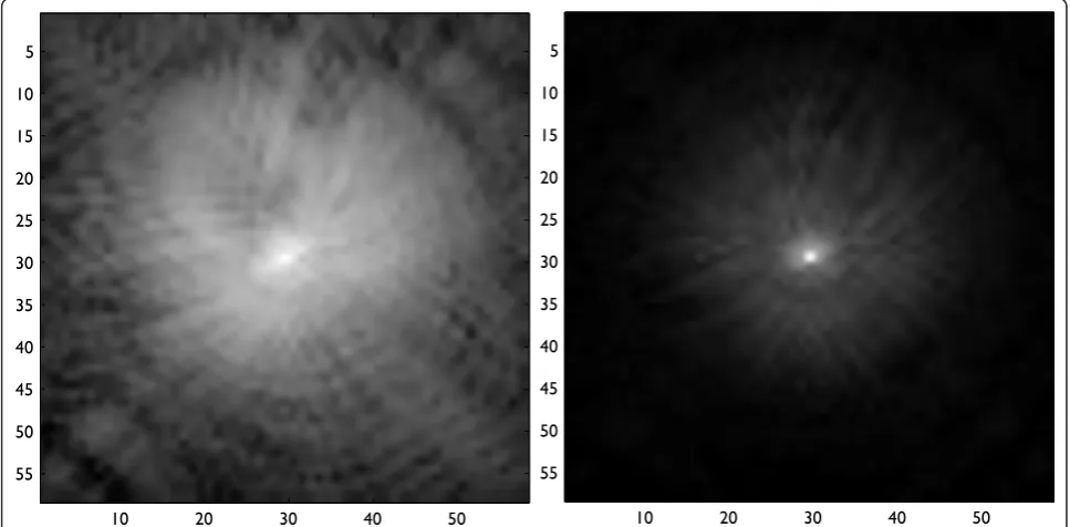
The third SV filter (BLUR3) tries to model a more realistic case: the aberrated PSFs of Hubble Space Telescope. Shortly after its deployment on April 24th 1990, a fabrication error in the 2.4 m primary mirror (PM) was discovered. The wide field and planetary camera (WFPC) is the principal instrument of the HST, occupying the central portion of the telescope’s focal plane. The HST suffered mainly from spherical aberration in the primary mirror. So, the aberration caused a strongly space-variant PSF. Restoration is further complicated by incomplete knowledge of the PSF and the time variance resulting from changes in focus and spacecraft motion. While the stars are almost ideal point sources, obtaining experimental PSFs is not a simple task. Image cannot be saturated so calibration experiments must be carefully designed, and the dependence on wavelength and the large
sensor size requires a huge amount of measures. So, a complete practical study of aberrations in WFPC was dismissed by the Spatial Agency, because the required observation time was not affordable. Nevertheless, PSF modeling programs, such as TinyTIM [28,29], have been very helpful for characterization and restoration of the images of all the instruments of the Hubble, in its different configurations for filters, wavelengths and even variations over time. Despite their limitations and simplifications assumed, these programs give us a good starting point. TinyTIM C source code is freely distrib-uted, so it can be compiled and executed on any machine.
The first WFPC consisted of two separate cameras, each comprising four 800×800 pixel Texas Instruments CCDs arranged to cover a contiguous field of view. We have modified TinyTIM C source code to fix some minor bugs and model a section of 256 ×256 pixels (the size of standard test images) and its associated PSFs in detector chip 1 of Wide Field Camera. The configura-tion was set as the one in 24th April 1991 (one year after the deployment) forf555w filter, object spectrum K4V and a null secondary despace (0.0 microns). The non-subsampled PSF size was 6.0 arc seconds, which leads to a discrete support of 58 ×58 pixels for each PSF. This simulation took one week on three computers working in parallel and generated 1.8 GB of data. Because of this heavy computational task, it could be considered to save all the possible PSFs to use them in a faster way, but the complete dataset for WFCP is esti-mated to require storage around 8 TB [30], and it should be recomputed each time the telescope is refo-cused. Hubble WFPC imaging seems to be a classic ill posed restoration problem, but it is a daunting challenge because the extension, variability in time and space, and lack of accuracy in PSF definitions. Here we only intend to use estimated PSFs as a means to compare different algorithms. The restoration of real images involves many more factors (e.g., Poissonian instead of Gaussian noise) that go beyond the scope of this article. Figure 2 shows the estimated PSFs for two different image sup-port locations.
We have used three classic 256×256 test images: Cam-eraman, House and Satellite. Cameraman and House are 256×256 8-bit gray-level standard test images. Satellite image was synthesized at the US Air Force Phillips Laboratory, Lasers and Imaging Directorate, Kirtland Air Force Base, New Mexico. It belongs to the Restore Tools toolbox data set [31].
In addition, three different amounts of white Gaussian noise have been added to the blurred images: low level (σ2=σ2
L = 0.308), medium (σM2 = 2), and high (σ2
As a first naïve approximation to boundary handling, all original images have been extended by mirroring its outer edges, prior to their SV-filtering. Of course, this is not a legitimate procedure to apply to real observations, because in these simulations filtering and noise addition have been applied also to the extended original image. At the end of the restoration, the previously added extra pixels are removed from the restored image, in order to obtain the same resolution as in the original. In addi-tion, at each iteration of L0-AbS, each convolution is done using mirror extension boundary conditions (note that, contrary to the extension of the original image, this intermediate mirror extension is legitimate). Rigor-ous treatment of boundary conditions is left as future study.
5.1.2 Image representation and training of statistical model parameters
In this study, we have used two frames for the non lin-ear method: a translation invariant version of the Haar pyramid (TIHP, quasi-Parseval), as described in [32], and the Dual-Tree Complex Wavelet Transform [26] which is a Parseval Frame, both with four scales.
As introduced in Section 4.3, the L0-AbS method leans on an image model using two statistical para-meters: aand sr. In this article, these parameters are estimated by optimizing the algorithm’s performance for a set of training images and degradations. We have cho-sen eight gray-scale images from USC-SIPI Image Data-base that represent natural scenes: Couple, Man, Bridge, Elaine, MoonSurface, ChemicalPlant, Pentagon and Aer-ial5.2.09; and two spatially variant blurring kernels: BLUR1 and BLUR2 (PSF support size is smaller than BLUR3 and faster to compute in spatial domain). Some of the reference images have a higher resolution than our test images, so in the training set we only have used the central portion of 256 × 256 pixels, without any
scaling. As figure of merit to be maximized we have used the average ISNR (increment in Signal-to-Noise Ratio), in decibels, of all the considered deblurring tests (two blurs, eight images), independently for each of the three noise levels considered. Whereas it may be argued that this is not an ideal quality measurement (for several reasons), it is nevertheless quite simple, and it seems to behave robustly enough for this purpose. We believe that in this case the overlapping of BLUR1 and BLUR2 in the training and test stages, though not being ideal, it is a justified decision in the context of achieving a rea-sonable tradeoff among computational cost, quality and generality. Note that the test images are different from the training images, and that the test blurs include a case not used in the training set (BLUR3).
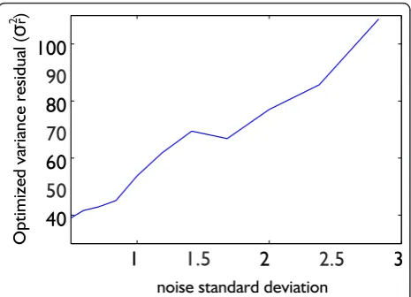
The optimization process has been computed inde-pendently for a range of noise levels froms2 = 0.25 to s2
= 8 in half octave intervals, as it is shown in Figure 3 for σr2 parameter. We have obtained the optimized values a= 4.52 andsr = 40.56 for low noise level,a= 8.31 and sr = 69.45 for medium noise level, and a = 15.07 andsr= 108.79 for high noise level.
The optimized image model parameter σr2 exhibits
an unexpected behavior, which has been consistently observed in further tests: it is approximately propor-tional to s (see Figure 3). Dependency of the opti-mized a on the noise variance, on the contrary, was much less pronounced. Making the image model para-meters to depend on the degradation parapara-meters does not fit a pure Bayesian estimation framework, for which the prior knowledge and the observation condi-tions are intrinsically independent. Within the empiri-cal Bayes approach, however, it is normal to adjust the prior features (in our case, the image model para-meters) depending on the amount and type of degrada-tion in the observadegrada-tion.c
5.1.3 Algorithm parameters spatially variant L0-AbS
There are two main parameters in the algorithm: the number of iterationsNiter in the spatially variant L0-AbS
algorithm and the numberJof reference kernels for the deformable filtering, both for the original PSFs and for the regularize inverse filtering (we have used the same valueJ’=J). In addition, one must choose a certain spa-tial support for the deformable kernels and their regu-larized inverse quadratic version ("the inverse kernels”, in short). In the first case the obvious choice is picking the maximal effective spatial support among all the PSFs. However, for the inverse kernel the effective sup-port will depend on the amount of regularization: the effective size will decrease as the regularization increases, and vice versa, because regularization increases the smoothness of the Fourier spectrum. As shown in Figure 1, we have chosen a square support of
1
2
3
40
60
80
100
noise standard deviation
50
70
90
1.5
2.5
Optimized variance residual (
σ
r
)
2
15 × 15 for the PSFs and of 29 × 29 for the inverse kernels.
We have observed that, similarly to what happened in the SI case, the L0-AbS method converges to a point near the MSE-optimum. It gets very close after a few steps, and then it moves slightly away but remains in the immediate vicinity. We have found a good compro-mise between speed and quality in the studied cases by takingNiter = 20.
As mentioned above, in many real cases there is a large amount of overlapping among (centered) PSFs, both in the direct and inverse regularized SV filtering. Therefore, the number J of regularized and inverted deformable kernels can be set quite small to reduce the number of convolutions without losing much accuracy.
The number of deformable kernels considered in the study cases is only J = 4, although it could be particu-larly tuned for each blur. This aspect is further studied in the Section 5.2.
As far as we have observed, the number of iterations has stronger influence than the number of deformable kernels on the final quality, provided that the number of deformable kernels is not too low. It is immediate to check that the complexity of the spatially variant L0-AbS method grows linearly with each of these parameters.
5.1.4 Algorithm parameters in HyBR and sectional methods
The examples of RestoreTools Toolbox [31] are limited to a small subset of PSFs, so that degradation is mod-eled as a set of locally spatially invariant regions. It
50 100 150 200 250
40 60 80 100 120 140 160
Number of considered eigenvectors
decibels
SNR between “inverse kernels” and their approximations
SNR(Hi0,Hi0aprox) with BLUR1
SNR(Hi0,Hi0aprox) with BLUR3
50 100 150 200 250
40 60 80 100 120 140 160
Number of considered eigenvectors
decibels
SNR between PSFs and their approximations
SNR(H0,H0aprox) with BLUR1
SNR(H0,H0aprox) with BLUR3
resembles to sectional methods although HyBR algo-rithm is more flexible. When the number of PSFs increases memory needs grow dramatically, and the ori-ginal code cannot be run. Therefore, we have slightly modified the HyBR code in order to support real spa-tially variant PSFs in an efficient way, even with an arbi-trary number of PSFs. In our case, a different PSF is associated to each pixel in the images. No pre-condi-tioning has been applied.
For the sectional method [12] we have defined 8×8 = 64 uniform regions, so each local invariant region is only 32×32 pixels. For each region it applies a classical FFT-based Wiener filtering. Obviously, this method should give better results than the application of a glo-bal Wiener filtering on the complete image, because it is approximately adapted to the filtering at each region. Only the central PSF of each region is considered in the restoration. Its computational performance grows super-linearly with the number of processed regions in multi-core implementations thanks to the effect of memory hierarchy in the small test images we used.
5.2 Two study cases
In this section, we study in some depth how the described deformable filtering techniques have been applied in two SV filtering cases: BLUR1 (synthetic scaled radial PSFs) and BLUR3 (Hubble PSFs).
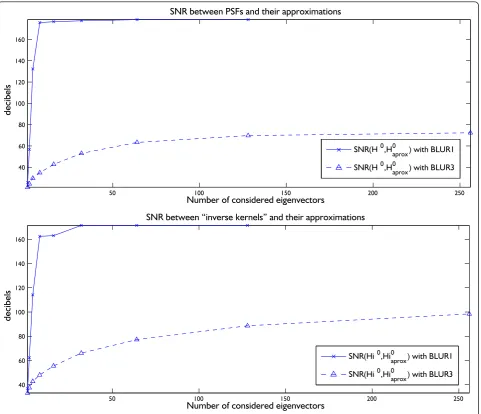
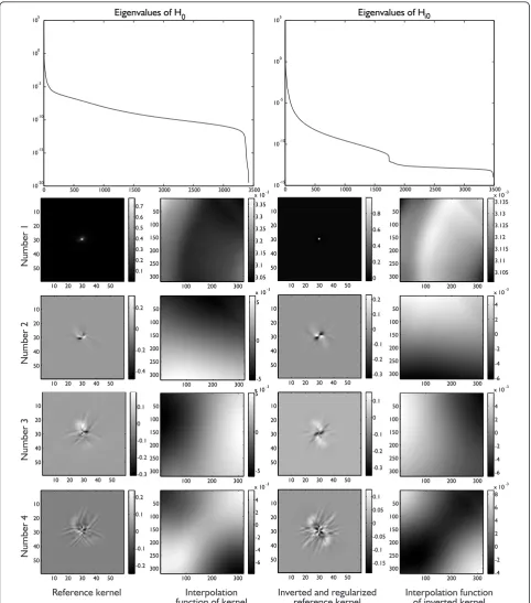
The PSF field in BLUR1 is quite smooth, according to Equation 15. So, as expected, it shows a significant amount of overlapping among centered PSFs, and, therefore, a small effective dimensionality of its matrix of stacked, centered at zero, PSFs. From Figures 1 and 4a, we can see thatJ= 4 is more than enough to obtain a high accuracy in all the SV-filtering stages.
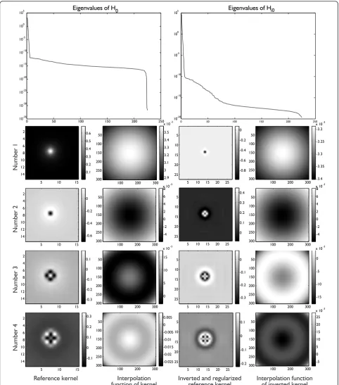
The eigenvalues of H0 are represented in the top left
of Figure 1. They fall steeply more than 12 orders of magnitude. Most of the energy is concentrated in a few singular vectors. Figure 4 shows the SNR between the matrix of stacked PSFs centered at zero and its approxi-mation with a number of eigenvectors. Such behavior is shared by the inverse kernel case (top right).
The first column in the lowest part of Figure 1 shows the reference kernels, and the second column their interpolation functions along the image. These interpo-lation functions shows the local weight of each reference kernel in the image (in the figure without taking into account the eigenvalue weight, for visualization sake).
It is easy to appreciate that the main reference kernel has a shape similar to the original radial PSF (like an average of all of them), whose influence is more impor-tant in the center of the image. The second one reminds a first derivative of this shape, it may be positive or negative weighted to approximate the extension of each PSF. The remaining ones help to define the subtle
details to capture the variability of the original PSFs [33]. Their relative influences -as seen in the interpola-tion funcinterpola-tions- show a more complex radial character.
Right columns, in Figure 1, have the four first inverse regularized deformable kernels and their interpolation functions. Although the nature of these PSFs is different, a similar pattern is observed.
A similar analysis is presented in Figure 5 for BLUR3. The PSFs correspond to a region of 256×256 pixels in chip0 of the WFPC of Hubble Space Telescope in the configuration of 24th April 1991. The degradation is quite variant. Most of the energy is located in only a few elements again (top left), but it does not fall so sharply as in the previous case. Because of this, we need more deformable kernels to approximate the original PSFs accurately (Figure 4). Four main direct and inverse deformable kernels are represented in columns 1 and 3 with linear contrast, so secondary lobes are not high-lighted. They are nonsymmetric and rather different from the original ones (Figure 2). The influence of these kernels take different directions as it is illustrated by the interpolation functions.
In the following section, the number of deformable kernels has been cut toJ = 4 to show the robustness of the algorithm in a set of representative scenarios, even in cases where very few filters are applied.
5.3 Results
Figures 6, 7, 8, and 9 show some comparative visual examples of our method’s performance, for different blurs and noise levels, for the three considered images. The improvement of visual quality with respect to the observation and also with respect to the competitors is outstanding. Probably, the most relevant difference with the compared methods is the much more powerful noise removal, whereas edges and other salient features in the images are, in general, substantially better re-gen-erated. This is clearly reflecting the much higher perfor-mance of non-linear methods compared to classical linear approaches.
Tables 1, 2, and 3 show average (and standard devia-tion, for 16 different noise realizations) Increment in Signal-to-Noise Ratio, in decibels, for the three differ-ent implemdiffer-ented SV blurs (respectively), the three images and the three noise levels. Results are com-pared to the two methods used as reference here. Overall, the improvement is very strong. As simulated observations where extended beyond the original images boundaries, we have applied the same post-cut-ting of the valid area after the estimation for all three compared methods.
0 50 100 150 200 250 10-35 10-30 10-25 10-20 10-15 10-10 10-5 100
105 Eigenvalues of H0
0 50 100 150 200 250
10-20 10-15 10-10 10-5 100
105 Eigenvalues of Hi0
Number 1
Number 4
Number 3
Number 2
Reference kernel Interpolation
function of kernel Inverted and regularized reference kernel Interpolation functionof inverted kernel
5 10 15
2 4 6 8 10 12 14 0.1 0.2 0.3 0.4 0.5 0.6
5 10 15
2 4 6 8 10 12 14 -0.6 -0.4 -0.2 0
5 10 15
2 4 6 8 10 12 14 -0.1 0 0.1 0.2 0.3 2 4 6 8 -0.1 0 0.1
5 10 15
10
12
14 -0.3
-0.2
5 10 15 20 25 5 10 15 20 25 -0.8 -0.6 -0.4 -0.2 0
5 10 15 20 25 5 10 15 20 25 0 0.1 0.2 0.3 0.4
5 10 15 20 25 5 10 15 20 25 -0.3 -0.2 -0.1 0
5 10 15 20 25 5 10 15 20 25 -0.2 -0.1 0 0.1 100 200 300
50 100 150 200 250 300 2.9 3 3.1 3.2 3.3 3.4 3.5 x 10⁻³
100 200 300 50 100 150 200 250 300 -4 -2 0 2 4 6 8 x 10⁻³
100 200 300 50 100 150 200 250 300 0 5 10 15 x 10-3
100 200 300 50 100 150 200 250 300 -0.025 -0.02 -0.015 -0.01 -0.005 0 0.005
100 200 300 50 100 150 200 250 300 -3.4 -3.35 -3.3 -3.25 -3.2 x 10⁻³
100 200 300 50 100 150 200 250 300 -4 -2 0 2 4 6 8 x 10⁻³
50
100
150
-5 0 x 10-3
100 200 300 200
250
300
-15 -10
100 200 300 50 100 150 200 250 300 -5 0 5 10 15 20 25 x 10-3
0 500 1000 1500 2000 2500 3000 3500 10-20 10-15 10-10 10-5 100
105 Eigenvalues of H0
0 500 1000 1500 2000 2500 3000 3500 10-15
10-10 10-5 100
105 Eigenvalues of Hi0
Number 1
Number 4
Number 3
Number 2
Reference kernel Interpolation
function of kernel Inverted and regularized reference kernel Interpolation functionof inverted kernel
10 20 30 40 50 10 20 30 40 50 0.1 0.2 0.3 0.4 0.5 0.6 0.7
10 20 30 40 50 10 20 30 40 50 -0.4 -0.2 0 0.2 10 0.1
10 20 30 40 50 20 30 40 50 -0.3 -0.2 -0.1 0
10 20 30 40 50 10 20 30 40 50 -0.2 -0.1 0 0.1 0.2
100 200 300 50 100 150 200 250 300 3.05 3.1 3.15 3.2 3.25 3.3 3.35 x 10⁻³
100 200 300 50 100 150 200 250 300 -5 0 5 x 10⁻³
100 200 300 50 100 150 200 250 300 -5 0 5 x 10⁻³
100 200 300 50 100 150 200 250 300 -6 -4 -2 0 2 4 x 10⁻³
10 20 30 40 50 10 20 30 40 50 0 0.2 0.4 0.6 0.8
10 20 30 40 50 10 20 30 40 50 -0.3 -0.2 -0.1 0 0.1 0.2
10 20 30 40 50 10 20 30 40 50 -0.3 -0.2 -0.1 0 0.1
10 20 30 40 50 10 20 30 40 50 -0.15 -0.1 -0.05 0 0.05 0.1
100 200 300 50 100 150 200 250 300 3.105 3.11 3.115 3.12 3.125 3.13 3.135 x 10⁻³
100 200 300 50 100 150 200 250 300 -6 -4 -2 0 2 4 x 10⁻³
100 200 300 50 100 150 200 250 300 -6 -4 -2 0 2 4 x 10⁻³
100 200 300 50 100 150 200 250 300 -4 -2 0 2 4 6 8 x 10⁻³
Figure 6Top left: Original Cameraman test image. Top right: Degraded image with BLUR2 and medium amount of additive gaussian noise (σ2
Figure 7 Top left: Original Satellite test image. Top right: Degraded image with BLUR1 and small amount of additive gaussian noise
σ2
M= 0.308
Figure 8Top left: Original Satellite test image. Top right: Degraded image with BLUR3 and a medium amount of additive gaussian noise (σ2
Figure 9 Top left: Original House test image. Top right: Degraded image with BLUR3 and a large amount of additive gaussian noise
σ2
M= 8
Quad core Xeon E5504 CPUs and 16 GB of main mem-ory. Although the sectional method is a bit faster, over-all times of the three methods are in the same range. We consider this a notable achievement, as our method is non-linear and iterative, so conceptually much more complex (which clearly translates into a superior MSE-performance, as we have seen) than the compared linear ones. Execution times and main memory requirements are notably higher in BLUR3 than in the other degrada-tion cases in our method. This is due to the fact that the expressionHTyin step 4 must be explicitly calcu-lated as a sparse matrix-vector multiplication (not like a deformable filtering), because Hubble PSFs are not so spectrally concentrated as BLUR1 and BLUR2 (as it is shown in Figures 4b and 5).
6 Conclusions and future study
Many real imaging processes involve SV linear degrada-tion. Thus, a single PSF is not enough to characterize the blur in the observation model, and a local PSF for each spatial location must be considered. In this study, a least squares optimal deformable filtering approximation is introduced as an efficient tool for linear SV filtering, in the
context of restoring SV-degraded images. Based on this technique a new formalism for linear SV operators has been proposed, that highlights difference between IKs and PSFs. This formalism helped us to formulate an efficient way to implement the transposed SV-filtering based uniquely on the PSFs. We also have proposed a method for implementing an approximation of the filtering of a SV-matrix regularized inverted, under the assumption of having smoothly varying kernels, and enough regulariza-tion. We applied these techniques to implement a SV-ver-sion of a recent successful sparsity-based image deconvolution method. A high performance (high speed, high visual quality and low mean squared error, MSE) is demonstrated through several simulation experiments (one of them based on the Hubble telescope PSFs), by comparison to two state-of-the-art methods. As a initial test, synthetic star cluster images have been processed with the same set of obtained parameters for natural images, in order to check optimized parameters’ robust-ness in a case with a very different image statistics. Results were comparable to the ones obtained with other meth-ods. We have also adapted the underlying statistical model by proper training with typical real astronomical images (from Kitt Peak observatory) with different blurs and noise levels; as we expected in this case, results are clearly better than the previous ones (in a range between 1 and 3 dBs). So, it is recommended to choose properly statistical para-meter values to achieve a very high-performance in each application (astronomical data, natural images in photo-graphy, microphoto-graphy, medical images, etc.).
Whereas we have used the SVD as a key tool for the proposed SV-filtering techniques, the fact of using it over the set of centered PSFs, instead of on the PSFs at their original locations, as previous studies have done, makes a huge difference in efficiency and accuracy terms. By means of this extra degree of efficiency, for a given accu-racy, we have been able to include these SV-filtering tech-niques as part of an iterative non-linear deblurring Table 1 Averaged ISNR of restored images with several
noise levels with BLUR1
Image Method BLUR1
σ2
L = 0.308 σM2 = 2 σH2= 8 HyBR 6.39±0.03 -1.51±0.04 0.49±0.06 Cameraman Trussell 6.73±0.03 0.71±0.02 -1.45±0.03 var. L0AbS 12.76±0.04 8.90±0.02 6.49±0.05 HyBR 2.33±0.03 -5.65±0.04 -3.76±0.08
House Trussell 2.82±0.03 -2.84±0.03 -4.30±0.03 var. L0AbS 11.13±0.03 8.43±0.03 6.69±0.05 HyBR 6.99±0.03 5.81±0.01 3.74±0.02
Satellite Trussell 7.61±0.04 2.17±0.02 0.65±0.03 var. L0AbS 15.79±0.06 9.73±0.09 6.73±0.05
Table 2 Averaged ISNR of restored images with several noise levels with BLUR2
Image Method BLUR2
σ2
L = 0.308 σM2 = 2 σH2= 8 HyBR 3.07±0.00 2.30±0.00 1.72±0.01 Cameraman Trussell 0.05±0.03 0.69±0.03 0.83±0.02 var. L0AbS 4.21±0.01 3.27±0.02 2.63±0.02 HyBR 4.33±0.01 3.46±0.01 2.79±0.01
House Trussell -0.48±0.04 -0.26±0.05 -0.09±0.05 var. L0AbS 5.14±0.03 4.18±0.02 3.68±0.02 HyBR 2.77±0.00 1.97±0.00 1.43±0.01
Satellite Trussell 2.67±0.02 2.30±0.02 2.02±0.03 var. L0AbS 4.51±0.02 3.83±0.02 3.35±0.02
Table 3 Averaged ISNR of restored images with several noise levels with BLUR3
Image Method BLUR3
σ2
L = 0.308 σM2 = 2 σH2= 8 HyBR 8.66±0.03 0.77±0.02 -4.91±0.02 Cameraman Trussell 8.59±0.03 2.83±0.03 0.86±0.02 var. L0AbS 13.95±0.04 9.13±0.04 6.30±0.03 HyBR 5.44±0.04 -2.61±0.03 -8.10±0.01
House Trussell 5.68±0.03 0.05±0.03 -1.22±0.02 var. L0AbS 13.02±0.03 10.62±0.05 8.68±0.04 HyBR 9.73±0.03 7.06±0.04 4.83±0.02
method which is much more powerful than classical linear approaches, in a similar computation time.
As future study, it is still pending to explore efficient ways to deal with image boundaries. Finally, in this first part of the article we only deal with simulations, because of the complexity to process real images when the PSF field is unknown. The second part of this arti-cle provides an in-depth study with real astronomical data.
Endnotes a
Other SV-restoration techniques could benefit as well of the proposed techniques, e.g., adapting a classical Wiener restoration to a SV-blurred noisy degradation.
b
We have forced that all PSFs integrate to one. This is the reason of using “∞” instead of“ =“ in their defini-tions. cAn in-depth analysis of this issue lies beyond the scope of this article. However, a partial explanation of the observed behavior is that the image model para-meters are also estimated from the observation, and, as such, they are subject to error. The bias-variance trade-off in these estimates, empirically optimized in terms of the final image estimation performance, may shift a lot, depending on the observation conditions, even when the uncorrupted original remains the same.
Acknowledgements
We thank Luis Pastor, Marcos Nobalvos, and Ángela Mendoza, from Universidad Rey Juan Carlos, for their support when our computer server broke down, and their thoughtful suggestions to port the code to a computer with strong main memory restrictions. This study was partially supported by the computing facilities of Extremadura Research Center for Advances Technologies (CETA-CIEMAT). The CETA-CIEMAT belongs to the Spanish Ministry of Science and Innovation. We also thank the EURASIP anonymous reviewers for their comments. DM had been funded by grant CICYT TIN2010-21289-C02-01. JP had been funded by grants CICYT TEC2009-13696 and CSIC PIE201050E021. All grants from the Spanish Education, and Science&Innovation Ministries. Computing facilities of Extremadura Research Center for Advances Technologies (CETA-CIEMAT) had been funded by the European Regional Development Fund (ERDF)
Author details
1E.T.S. Ingenieria Informatica, Universidad Rey Juan Carlos, Madrid, Spain 2
Instituto de Optica, Consejo Superior de Investigaciones Científicas, Madrid, Spain
Competing interests
The authors declare that they have no competing interests.
Received: 30 June 2011 Accepted: 3 May 2012 Published: 3 May 2012
References
1. G Golub, W Kahan, Calculating the singular values and pseudo-inverse of a matrix. Journal of the Society for Industrial and Applied Mathematics: Series B, Numerical Analysis.2, 205–224 (1965). doi:10.1137/0702016
2. H Andrews, C Patterson, Singular value decompositions and digital image processing. IEEE Transactions on Acoustics, Speech and Signal Processing. 24(1), 26–53 (Feb 1976). doi:10.1109/TASSP.1976.1162766
3. S Ben Hadj, L Blanc-Fraud, Restoration mehod for spatially variant blurred images. Research Report 7654, INRIA (June 2011)
4. AF Boden, DC Redding, RJ Hanisch, J Mo, Massively parallel spatially variant maximum-likelihood restoration of hubble space telescope imagery. J Opt Soc Am A.13(7), 1537–1545 (1996). doi:10.1364/JOSAA.13.001537 5. D Calvetti, B Lewis, L Reichel, Restoration of images with spatially variant
blur by the gmres method, inAdvanced Signal Processing Algorithms, Architectures, and Implementations X, ed. FT Luk, Proceedings of the Society of Photo-Optical Instrumentation Engineers (SPIE), San Diego, CA, USA,4116, 364–374 (November 2000)
6. J Chung, JG Nagy, DP OLeary, A weighted-gcv method for lanczos-hybrid regularization. Electronic Transactions on Numerical Analysis.28, 149–167 (2008)
7. TP Costello, WB Mikhael, Efficient restoration of space-variant blurs from physical optics by sectioning with modified wiener filtering. Digital Signal Processing.13(1), 1–22 (January 2003). doi:10.1016/S1051-2004(02)00004-0 8. L Denis, E Thiebaut, F Soulez, Fast model of space-variant blurring and its application to deconvolution in astronomy. in2011 18th IEEE International Conference on Image Processing (ICIP). Brussels 2817–2820 (Sep 2011) 9. DA Fish, J Grochmalicki, ER Pike, Scanning singular-value-decomposition
method for restoration of images with space-variant blur. J Opt Soc Am A. 13(3), 464–469 (1996). doi:10.1364/JOSAA.13.000464
10. G Nagy James, P O’Leary Dianne, Restoring images degraded by spatially-variant blur. SIAM J Sci Comput.19, 1063–1082 (1998). doi:10.1137/ S106482759528507X
11. N Hajlaoui, C Chaux, G Perrin, F Falzon, A Benazza-Benyahia, Satellite image restoration in the context of a spatially varying point spread function. J Opt Soc Am A.27(6), 1473–1481 (2010). doi:10.1364/JOSAA.27.001473 12. H Trussell, B Hunt, Image restoration of space-variant blurs by sectioned
methods. IEEE Transactions on Image Processing.26(6), 608–609 (December 1978)
Table 4 Averaged execution times (in seconds) for the applied algorithms in different images and noise levels.
Image Method BLUR1 BLUR2 BLUR3
σ2
L = 0.308 σM2 = 2 σH2= 8 σ
2
L = 0.308 σM2 = 2 σH2= 8 σ
2
L = 0.308 σM2 = 2 σH2= 8
HyBR 19.48 24.96 18.90 4.59 3.03 2.27 127.35 143.13 159.90
Cameraman Trussell 1.00 0.80 0.68 0.88 0.89 0.88 1.02 1.13 0.89
var. L0AbS 3.54 3.53 3.64 3.50 3.49 3.51 10.64 10.47 10.50
HyBR 16.99 21.47 19.27 3.48 2.47 1.79 120.34 139.24 158.00
House Trussell 1.02 0.87 0.83 0.75 0.89 0.96 0.99 0.97 1.12
var. L0AbS 3.91 3.90 3.91 3.51 3.52 3.50 10.70 10.62 10.65
HyBR 17.82 11.51 3.76 3.38 2.38 1.86 130.84 148.19 51.04
Satellite Trussell 0.89 0.71 0.91 0.81 0.88 0.95 1.12 0.97 1.06
var. L0AbS 3.91 3.90 3.92 3.51 3.51 3.53 10.65 10.58 10.60
13. G Nagy James, P O’Leary Dianne, Fast iterative image restoration with a space-varying psf. The International Society for Optical Engineering, editor, Advanced Signal Processing Algorithms, Architectures, and Implementations IV. Proceedings of the Society of Photo-Optical Instrumentation Engineers (SPIE). Bellingham.3162, 388–399 (1997)
14. Gene Golub, Charles Van Loan, Total least squares, inSmoothing Techniques for Curve Estimation, of Lecture Notes in Mathematics, vol. 757, ed. by Th Gasser, M Rosenblatt (Springer Berlin/Heidelberg, 1979), pp. 69–76. doi:10.1007/BFb0098490
15. P Perona, Deformable kernels for early vision. IEEE Transactions on Pattern Analysis and Machine Intelligence.17(5), 488–499 (May 1995). doi:10.1109/ 34.391394
16. A Tabernero, J Portilla, R Navarro, Duality of log-polar image representations in the space and spatial-frequency domains. IEEE Transactions on Signal Processing.47(9), 2469–2479 (1999). doi:10.1109/78.782190
17. R Lupton, JE Gunn, Z Ivezic, GR Knapp, S Kent, The sdss imaging pipelines, inAstronomical data analysis software and systems X: proceedings of a meeting held at Boston, Massachusetts, USA, 12-15 November 2000, Astronomical Society of the pacific, 2001,238, 269–279 (12–15 November 2000)
18. M Jarvis, B Jain, Principal component analysis of psf variation in weak lensing surveys. Arxiv preprint astroph/0412234 (2004)
19. Tim Schrabback, Jan Hartlap, Benjamin Joachimi, Martin Kilbinger, Patrick Simon, Karim Benabed, Marusa Bradac, Tim Eifler, Thomas Erben, D Fassnacht Christopher, F William High, Stefan Hilbert, Hendrik Hildebrandt, Henk Hoekstra, Konrad Kuijken, Phil Marshall, Yannick Mellier, Eric Morganson, Peter Schneider, Elisabetta Semboloni, Ludovic Van Waerbeke, Malin Velander, Evidence of the accelerated expansion of the universe from weak lensing tomography with COSMOS. Astronomy & Astrophysics.516, 1–26 (2010)
20. MJ Jee, JP Blakeslee, M Sirianni, AR Martel, RL White, HC Ford, Principal component analysis of the time-and position-dependent point-spread function of the advanced camera for surveys. Publications of the Astronomical Society of the Pacific.119(862), 1403–1419 (2007). doi:10.1086/524849
21. Per Christian Hansen, G Nagy James, P O’Leary Dianne, Deblurring Images: Matrices, Spectra, and Filtering (Fundamentals of Algorithms 3)
(Fundamentals of Algorithms), (Society for Industrial and Applied Mathematics, Philadelphia, PA, USA, 2006)
22. J Portilla, Image restoration through L0 analysis-based sparse optimization in tight frames. in16th IEEE International Conference on Image Processing (ICIP)3909–3912 (Nov 2009)
23. J Portilla, E Gil-Rodrigo, D Miraut, R Suarez-Mesa, CONDY: Ultra-fast high performance restoration using multi-frame L2-relaxed-L0 sparsity and constrained dynamic heuristics. in18th IEEE International Conference on Image Processing (ICIP).Brussels 1837–1840 (Sep 2011)
24. E Gil-Rodrigo, J Portilla, D Miraut, R Suarez-Mesa, Efficient joint poisson-gauss restoration using multi-frame L2-relaxed-L0 analysis-based sparsity. in 18th IEEE International Conference on Image Processing (ICIP).Brussels 1385–1388 (Sep 2011)
25. JW Goodman,Introduction to Fourier optics, (Roberts & Company Publishers, 2005)
26. N Kingsbury, Complex wavelets for shift invariant analysis and filtering of signals. Applied and Computational Harmonic Analysis.10(3), 234–253 (2001). doi:10.1006/acha.2000.0343
27. M Rerabek, P Páta, Advanced processing of astronomical images obtained from optical systems with ultra wide field of view. inProceedings of SPIE. 7443, 74431Z (2009)
28. J Krist, Tiny Tim: an HST PSF simulator, inAstronomical Data Analysis Software and Systems II, vol. 52, ed. by RJ Hanisch, RJV Brissenden, Barnes Jeannette (ADASS, 1993), pp. 536–539
29. J Krist, H Hasan, Deconvolution of HST WFPC images using simulated PSFs. inAstronomical Data Analysis Software and Systems II.52, 530–532 (1993) 30. RJ Hanisch, RL White, Hst image restoration: current capabilities and future
prospects [invited]. inVery High Angular Resolution Imaging.158, 61 (1994) 31. JG Nagy, K Palmer, L Perrone, Iterative methods for image deblurring: a
matlab object-oriented approach. Numerical Algorithms.36(1), 73–93 (2004) 32. JA Guerrero-Colón, L Mancera, J Portilla, Image restoration using
space-variant gaussian scale mixtures in over-complete pyramids. Image Processing, IEEE Transactions on.17(1), 27–41 (2008)
33. R Lauer Tod, Deconvolution with a spatially-variant PSF. Arxiv preprint astro-ph/0208247 (2002)
doi:10.1186/1687-6180-2012-100
Cite this article as:Miraut and Portilla:Efficient shift-variant image
restoration using deformable filtering (Part I).EURASIP Journal on Advances in Signal Processing20122012:100.
Submit your manuscript to a
journal and benefi t from:
7 Convenient online submission 7 Rigorous peer review
7 Immediate publication on acceptance 7 Open access: articles freely available online 7 High visibility within the fi eld
7 Retaining the copyright to your article