Iterative Decoding of Concatenated Codes: A Tutorial
Phillip A. Regalia
D´epartement Communications, Images et Traitement de l’ Information, Institut National des T´el´ecommunications, 91011 Evry Cedex, France
Department of Electrical Engineering and Computer Science, Catholic University of America, Washington, DC 20064, USA Email:[email protected]
Received 29 September 2003; Revised 1 June 2004
The turbo decoding algorithm of a decade ago constituted a milestone in error-correction coding for digital communications, and has inspired extensions to generalized receiver topologies, including turbo equalization, turbo synchronization, and turbo CDMA, among others. Despite an accrued understanding of iterative decoding over the years, the “turbo principle” remains elusive to master analytically, thereby inciting interest from researchers outside the communications domain. In this spirit, we develop a tutorial presentation of iterative decoding for parallel and serial concatenated codes, in terms hopefully accessible to a broader audience. We motivate iterative decoding as a computationally tractable attempt to approach maximum-likelihood decoding, and characterize fixed points in terms of a “consensus” property between constituent decoders. We review how the decoding algorithm for both parallel and serial concatenated codes coincides with an alternating projection algorithm, which allows one to identify conditions under which the algorithm indeed converges to a maximum-likelihood solution, in terms of particular likelihood functions factoring into the product of their marginals. The presentation emphasizes a common framework applicable to both parallel and serial concatenated codes.
Keywords and phrases:iterative decoding, maximum-likelihood decoding, information geometry, belief propagation.
1. INTRODUCTION
The advent of the turbo decoding algorithm for parallel con-catenated codes a decade ago [1] ranks among the most sig-nificant breakthroughs in modern communications in the past half century: a coding and decoding procedure of rea-sonable computational complexity was finally at hand offer-ing performance approachoffer-ing the previously elusive Shan-non limit, which predicts reliable communications for all channel capacity rates slightly in excess of the source entropy rate. The practical success of the iterative turbo decoding al-gorithm has inspired its adaptation to other code classes, no-tably serially concatenated codes [2,3], and has rekindled in-terest [4,5] in low-density parity-check codes [6], which give the definitive historical precedent in iterative decoding.
The serial concatenated configuration holds particular interest for communication systems, since the “inner en-coder” of such a configuration can be given more general interpretations, such as a “parasitic” encoder induced by a convolutional channel or by the spreading codes used in CDMA. The corresponding iterative decoding algorithm can then be extended into new arenas, giving rise to turbo
equal-This is an open access article distributed under the Creative Commons Attribution License, which permits unrestricted use, distribution, and reproduction in any medium, provided the original work is properly cited.
ization [7, 8,9] or turbo CDMA [10, 11], among doubt-less other possibilities. Such applications demonstrate the power of iterative techniques which aim to jointly opti-mize receiver components, compared to the traditional ap-proach of adapting such components independently of one another.
Interest in turbo decoding and related topics now ex-tends beyond the communications community, and has been met with useful insights from other fields; some references in this direction include [29] which draws on nonlinear sys-tem analysis, [30] which draws on computer science, in ad-dition to [31] (predating turbo codes) and [32] (more re-cent) which inject ideas from statistical physics, which in turn can be rephrased in terms of information geometry [33,34]. Despite this impressive pedigree of analysis techniques, the “turbo principle” remains difficult to master analytically and, given its fair share of specialized terminology if not a certain degree of mystique, is often perceived as difficult to grasp to the nonspecialist. In this spirit, the aim of this paper is to pro-vide a reasonably self-contained and tutorial development of iterative decoding for parallel and serial concatenated codes, in terms hopefully accessible to a broader audience. The pa-per does not aim at a comprehensive survey of available anal-ysis techniques and implementation tricks surrounding it-erative decoding (for which the texts [12,13,14] would be more appropriate), but rather chooses a particular vantage point which steers clear of unnecessary sophistication and avoids approximations.
We begin inSection 2by reviewing optimum (maximum a posteriori and maximum-likelihood) decoding of parallel concatenated codes. We motivate the turbo decoding algo-rithm as a computationally tractable attempt to approach maximum-likelihood decoding. A characterization of fixed points is obtained in terms of a “consensus” property be-tween the two constituent decoders, and a simple proof of the existence of fixed points is obtained as an application of the Brouwer fixed point theorem.
Section 3 then reexamines the calculation of marginal distributions in terms of a projection operator, leading to a compact formulation of the turbo decoding algorithm as an alternating projection algorithm. The material of the section aims at a concrete transcription of ideas originally developed by Richardson [29]; we include in addition a minimum-distance property of the projector in terms of the Kullback-Leibler divergence, and review how the turbo decoding algo-rithm indeed converges to a maximum-likelihood solution whenever specific likelihood functions factor into the prod-uct of its marginals. The factorization is known [18] to hold in extreme signal-to-noise ratios.
Section 4shows that the iterative decoding algorithm for serial concatenated codes also admits an alternating pro-jection interpretation, allowing us to transcribe all results for parallel concatenated codes to their serial concatenated counterparts. This should also facilitate unified studies of both code classes. Concluding remarks are summarized in Section 5.
2. TURBO DECODING OF PARALLEL CONCATENATED CODES
We begin by reviewing the classical turbo decoding algorithm for parallel concatenated codes. For simplicity, we restrict our development to the binary signaling case; them-ary case can
Systematic
encoder 1 (ξ1,. . .,ξk,η1,. . .,ηn−k)
(ξ1,. . .,ξk,ζ1,. . .,ζn−k) ξ=(ξ1,. . .,ξk)
Systematic encoder 2
Information bits
Parity-check bits
Figure1: Parallel concatenated encoder structure.
Systematic encoder 1 ξ=(ξ1,. . .,ξk)
Systematic encoder 1
Permu-tation
Systematic encoder 2
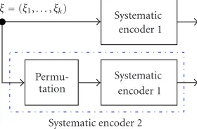
Figure2: Particular realization of the second encoder by using the first encoder with an interleaver.
be handled by direct extension (see, e.g., [24] for a particu-larly clear treatment) or by mapping them-ary constellation back to its binary origins.
To begin, a binary (0 or 1) information block ξ = (ξ1,. . .,ξk) is passed through two constituent encoders, as in Figure 1, to create two codewords:
ξ1,. . .,ξk,η1,. . .,ηn−k, ξ1,. . .,ξk,ζ1,. . .,ζn−k. (1) Both encoders are systematic and of ratek/n, so that the in-formation bitsξ1,. . .,ξkare directly available in either code-word. Note also that the two encoders need not share a com-mon rate, although we will adhere to this case for ease of no-tation.
In practice, an expedient method of realizing the second systematic encoder is to permute (or interleave) the infor-mation bitsξiand duplicate the first encoder, as inFigure 2. Since this is a particular instance ofFigure 1, we will simply consider two separate encodings ofξ =(ξ1,. . .,ξk) in what follows and avoid explicit reference to the interleaving op-eration, despite its importance in the study of the distance properties of concatenated codes [35].
The encoder outputs are converted to antipodal signal-ing (±1) and transmitted over a channel containing additive noise, giving the received signalsxi,yi, andzi:
xi=2ξi−1+bx,i, i=1, 2,. . .,k; yi=2ηi−1+by,i, i=1, 2,. . .,n−k; zi=2ζi−1+bz,i, i=1, 2,. . .,n−k.
(2)
signals into the vectors
x=
x1 .. . xk
, y=
y1 .. . yn−k
, z=
z1 .. . zn−k
. (3)
2.1. Optimum decoding
The maximum a posteriori decoding rule aims to calculate the a posteriori probability ratios
Prξi=1|x,y,z
Prξi=0|x,y,z, i=1, 2,. . .,k, (4)
with the decision rule favoring a 1 for theith bit if this ratio is greater than one, and 0 if the ratio is less than one. By using Bayes’s rule, each ratio can be developed as
Prξi=1|x,y,z
Prξi=0|x,y,z =
ξ:ξi=1Pr(ξ|x,y,z) ξ:ξi=0Pr(ξ|x,y,z) = ξ:ξi=1p(x,y,z|ξ) Pr(ξ)
ξ:ξi=0p(x,y,z|ξ) Pr(ξ) ,
(5)
involving the a priori probability mass function Pr(ξ) and the likelihood functionp(x,y,z|ξ), which is evaluated for the re-ceivedx,y, andzas a function of the candidate information bitsξ = (ξ1,. . .,ξk); the sum in the numerator (resp., de-nominator) is over all the configurations of the vectorξfor which theith bit is a “1” (resp., “0”). Since the noise samples are assumed independent, the likelihood function naturally factors as
p(x,y,z|ξ)=p(x|ξ)p(y|ξ)p(z|ξ). (6) For the Gaussian noise case considered here, the three likeli-hood evaluations appear as
p(x|ξ)∼exp
−x−cx(ξ)2 2σ2
,
p(y|ξ)∼exp
−y−cy(ξ)
2
2σ2
,
p(z|ξ)∼exp
−z−cz(ξ)2 2σ2
,
(7)
wherecx(ξ),cy(ξ), andcz(ξ) contain the antipodal symbols ±1 which would be received as a function of the candidate in-formation bitsξ, in the absence of noise. For non-Gaussian noise, the likelihood functions would, of course, assume dif-ferent forms.
The a posteriori probability ratios may therefore be writ-ten as
Prξi=1|x,y,z
Prξi=0|x,y,z=
ξ:ξi=1p(x|ξ)p(y|ξ)p(z|ξ) Pr(ξ) ξ:ξi=0p(x|ξ)p(y|ξ)p(z|ξ) Pr(ξ) ,
i=1, 2,. . .,k.
(8)
If the a priori probability mass function Pr(ξ) is uniform (i.e., Pr(ξ)=1/2kfor allξ), then this reduces to the maximum-likelihood decision metric:
Prξi=1|x,y,z
Prξi=0|x,y,z
= ξ:ξi=1p(x|ξ)p(y|ξ)p(z|ξ) ξ:ξi=0p(x|ξ)p(y|ξ)p(z|ξ)
if Pr(ξ) is uniform. (9)
If this expression were evaluated as written, the complexity of an optimum decision rule would beO(2k), since there are 2k configurations of thekinformation bits comprisingξ, lead-ing to as many likelihood function evaluations. This clearly becomes impractical for sizablek.
Observe now that if we instead consider an optimum de-coding rule using only one of the constituent encoders, we may write, by a development parallel to that above,
Prξi=1|x,y
Prξi=0|x,y =
ξ:ξi=1p(x|ξ)p(y|ξ)Pr(ξ) ξ:ξi=0p(x|ξ)p(y|ξ)Pr(ξ)
, (10)
Pr(ξi=1|x,z) Pr(ξi=0|x,z)=
ξ:ξi=1p(x|ξ)p(z|ξ)Pr(ξ) ξ:ξi=0p(x|ξ)p(z|ξ)Pr(ξ)
. (11)
If each constituent encoder implements a trellis code, thenx
andyform a Markov chain, as doxandz; the complexity of either decoding expression can then be reduced toO(k) by using the forward-backward algorithm from [36] (which, in turn, is a particular case of the sum-product algorithm [27]). If the a priori probability function Pr(ξ) is indeed uni-form, then it weighs all terms in the numerator and de-nominator equally and, as such, is effectively relegated to an unused variable in either decoding expression (10) or (11). Rather than accepting this status, one can imagine replacing the a priori probability function Pr(ξ), or “usurping” its po-sition, by some other function in an attempt to “bias” either decoding rule (10) or (11) towards the maximum-likelihood decoding rule in (9). In particular, if Pr(ξ) were replaced by p(z|ξ) in (10), or by p(y|ξ) in (11), then either expression would agree formally with (9).
In order to retain theO(k) complexity of the forward-backward algorithm from [36], however, the a priori proba-bility function Pr(ξ) is assumed to factor into the product of its bitwise marginals:
Pr(ξ)=Prξ1
Prξ2
· · ·Prξk. (12)
The likelihood function p(y|ξ) or p(z|ξ) does not, on the other hand, generally factor into its bitwise marginals, that is,
p(y|ξ)=py|ξ1
py|ξ2
· · ·py|ξk. (13)
the likelihood function p(y|ξ) or p(z|ξ) by a function that does factor into the product of its marginals. Many candidate approximations may be envisaged; that which has proved the most useful relies on extrinsic information values, which are reviewed next.
2.2. Extrinsic information values
We reexamine the likelihood function for the systematic bits:
p(x|ξ)= √ 1 2πσkexp
− k
i=1
xi−2ξi−12 2σ2
=k i=1
exp−xi−2ξi−12/2σ2 √
2πσ =px1|ξ1
px2|ξ2
· · ·pxk|ξk.
(14)
This shows that the likelihood function p(x|ξ) for the sys-tematic bits factors into the product of its marginals,1 just like the a priori probability mass function:
Pr(ξ)=Prξ1
Prξ2
· · ·Prξk. (15) Owing to these factorizations, each term from the numer-ator of (10) contains a factor p(xi|ξi = 1) Pr(ξi = 1), and each term from the denominator contains a factorp(xi|ξi= 0) Pr(ξi = 0). By isolating these common factors, we may rewrite the ratio from (10) as
Prξi=1|x,y
Prξi=0|x,y
= p
xi|ξi=1 pxi|ξi=0
intrinsic information
Prξi=1 Prξi=0
a priori information
× ξ:ξi=1p(y|ξ)
j=ipxj|ξjPrξj ξ:ξi=0p(y|ξ)
j=ipxj|ξj) Prξj
extrinsic information
.
(16)
The three terms on the right-hand side may be interpreted as follows:
(i) the first term indicates what theith received bitxi con-tributes to the determination of theith transmitted bit ξi; hence the name “intrinsic information.” It coincides with the maximum-likelihood metric for determining theith bit when no coding is used,
(ii) the second term expresses the a priori probability ratio for theith bit, and will be usurped shortly,
(iii) the third term expresses what the remaining bits in the packet (i.e., of indexj =i) contribute to the determi-nation of theith bit; hence the name “extrinsic infor-mation.”
1Although we show this factorization here for a Gaussian channel, the factorization holds, of course, for any memoryless channel model.
LetT(ξ)=T1(ξ1)T2(ξ2)· · ·Tk(ξk) be a factorable prob-ability mass function whose bitwise ratios are chosen to match the extrinsic information values above:
Tiξi=1 Tiξi=0
= ξ:ξi=1p(y|ξ)
j=ipxj|ξjPrξj ξ:ξi=0p(y|ξ)
j=ipxj|ξjPrξj, i=1, 2,. . .,k. (17)
Since these values depend on the likelihood function p(y|ξ) (in addition to the systematic bits save for xi), we may considerT(ξ) a factorable function which approximates, in some sense, the likelihood function p(y|ξ). (We will see in Theorem 2a condition under which this approximation be-comes exact). We now letT(ξ) usurp the place reserved for the a priori probability function Pr(ξ) (denoted Pr(ξ) ← T(ξ)) in the evaluation of the second decoder (11); since both p(x|ξ) andT(ξ) factor into the product of their respective marginals, we have
ξ:ξi=1p(x|ξ)p(z|ξ) Pr(ξ) ξ:ξi=0p(x|ξ)p(z|ξ) Pr(ξ)
←− ξ:ξi=1p(x|ξ)p(z|ξ)T(ξ) ξ:ξi=0p(x|ξ)p(z|ξ)T(ξ)
= p
xi|ξi=1 pxi|ξi=0
intrinsic information
Tiξi=1 Tiξi=0
pseudoprior
× ξ:ξi=1p(z|ξ)
j=ipxj|ξjTjξj ξ:ξi=0p(z|ξ)
j=ipxj|ξjTjξj
extrinsic information
.
(18)
Here we adopt the term “pseudoprior” for T(ξ) since it usurps the a priori probability function; similarly, the re-sult of this substitution may be termed a “pseudoposterior” which usurps the true a posteriori probability ratio.
Let nowU(ξ)=U1(ξ1)U2(ξ2)· · ·Uk(ξk) denote another factorable probability function whose bitwise ratios match the extrinsic information values furnished by this second de-coder:
Uiξi=1 Uiξi=0
= ξ:ξi=1p(z|ξ)
j=ipxj|ξjTjξj ξ:ξi=0p(z|ξ)
j=ipxj|ξjTjξj, i=1, 2,. . .,k. (19)
Systematic Parity-check
extrinsic Pseudoprior p(x|ξ)
p(y|ξ) U(m)
U(m+1)
D T(m)
1st decoder
2nd decoder Pseudoprior Parity-check extrinsic
Systematic
p(z|ξ) p(x|ξ)
Figure3: Flow graph of the turbo decoding algorithm.
the two decoders admits an external description as
pxi|ξi=1 pxi|ξi=0
U(m) i (1) U(m)
i (0) T(m)
i (1) T(m)
i (0)
= ξ:ξi=1p(y|ξ)p(x|ξ)U(m)(ξ) ξ:ξi=0p(y|ξ)p(x|ξ)U(m)(ξ) ,
(20)
pxi|ξi=1 pxi|ξi=0
T(m) i (1) T(m)
i (0) U(m+1)
i (1) U(m+1)
i (0)
= ξ:ξi=1p(z|ξ)p(x|ξ)T(m)(ξ) ξ:ξi=0p(z|ξ)p(x|ξ)T(m)(ξ) ,
(21)
in which (20) furnishesT(m)(ξ) and (21) furnishesU(m+1)(ξ). This is depicted in Figure 3. A fixed point corresponds to U(m+1)(ξ)=U(m)(ξ) which, by inspection of the pseudopos-teriors above, yields the following property.
Property1. A fixed point is attained if and only if the two de-coders yields the same pseudoposteriors (the left-hand sides of (20) and (21)) fori=1, 2,. . .,k.
A fixed point is therefore reflected by a state of “consen-sus” between the two decoders [15,29,37].
2.3. Existence of fixed points
A necessary (but not sufficient) condition for the algorithm to converge is that a fixed point exist, reflected by a state of consensus according toProperty 1. A convenient tool in this direction is the Brouwer fixed point theorem [38], which as-serts that any continuous map from a closed, bounded, and convex set into itself admits a fixed point; its application in the present context gives the following result [18,29].
Theorem 1. The turbo decoding algorithm from(20)and(21)
always admits a fixed point.
To verify, consider the pseudopriorsU(m)(ξi) evaluated forξi=1, which, at any iterationm, are (pseudo-) probabil-ities lying between 0 and 1:
0≤U(m)(1)≤1, i=1, 2,. . .,k. (22)
This clearly gives a closed, bounded, and convex set. Since the updated pseudopriors U(m+1) also lie in this set, and since the map fromU(m)(ξ) toU(m+1)(ξ) is continuous [18,29], the conditions of the Brouwer theorem are satisfied, to show existence of a fixed point.
3. PROJECTIONS AND PRODUCT DISTRIBUTIONS
A key element of the development thus far concerns the cal-culation of bitwise marginal ratios which, according to [20], provide the troublesome element which accounts for the dif-ference between a provably convergent algorithm [20] which is not practically implementable, and the implementable— but difficult to grasp—turbo decoding algorithm. We de-velop here an alternate viewpoint of the calculation of bitwise marginals in terms of a certain projection operator, adapted from the seminal work of Richardson [29].
Letq(ξ) be a distribution, for example, a probability mass function, or a likelihood function, which assigns a nonnega-tive number to each of the 2kevaluations ofξ=(ξ1,. . .,ξk). We letqbe the vector built from these 2kevaluations:
q=
qξ=(0,. . ., 0, 0) qξ=(0,. . ., 0, 1)
.. .
qξ=(1,. . ., 1, 1)
2kevaluations. (23)
We assume thatqis scaled such that its entries sum to one. The k marginal distributions determined from q(ξ), each having two evaluations at ξi = 0 andξi = 1 (1 ≤ i ≤ k), are given by
q1
ξ1=0
=
ξ:ξ1=0
q(ξ), q1
ξ1=1
=
ξ:ξ1=1
q(ξ),
q2
ξ2=0
=
ξ:ξ2=0
q(ξ), q2
ξ2=1
=
ξ:ξ2=1
q(ξ),
..
. ...
qkξk=0= ξ:ξk=0
q(ξ), qkξk=1= ξ:ξk=1
q(ξ). (24)
Definition1. The distributionq(ξ) is aproduct distributionif it coincides with the product of its marginals:
q(ξ)=q1
ξ1
q2
ξ2
· · ·qkξk. (25) The set of all product distributions is denoted byP.
It is straightforward to check thatq(ξ)∈P if and only if its vector representation is Kronecker decomposable as
q=q1⊗q2⊗ · · · ⊗qk (26)
with
qi= qi
ξi=0 qiξi=1
!
We note also thatP is closed under multiplication: ifq(ξ) andr(ξ) belong toP, so does their product:
s(ξ)=αq(ξ)r(ξ)∈P, (28) where the scalar αis chosen so that the evaluations ofs(ξ) sum to one. This operation can be expressed in vector nota-tion using the Hadamard (or term-by-term) product:
s=αqr. (29)
To simplify notations, the scalarαwill not be explicitly indi-cated, with the tacit understanding that the elements of the vector must be scaled to sum to one; we will henceforth write
s=qr, omitting explicit mention of the scale factorα. Suppose now r(ξ) is not a product distribution. If r1(ξ1),. . .,rk(ξk) denote its marginal distributions, then we can set
q(ξ)=r1
ξ1
r2
ξ2
· · ·rkξk, (30) to create a product distribution q(ξ) ∈ P which, by con-struction, generates the same marginals asr(ξ):
qiξi=riξi, i=1, 2,. . .,k. (31) This operation will be denoted by
q=π(r). (32)
We can observe thatqis a product distribution (q∈ P) if and only ifπ(q)=q, and sinceπ(r)∈Pfor any distribution
r, we must haveπ(π(r))=π(r), so thatπ(·) is a projection operator.
Definition2. The distributionqis the projection ofrintoP if (i)q∈P and (ii)qi(ξi)=ri(ξi).
The following section details some simple information-theoretic properties which reinforce the interpretation as a projection.
3.1. Information-theoretic properties of the projector
The results summarized in this section may be understood as concrete transcriptions of ultimately deeper results from the field of information geometry [33,34]. To begin, we recall that the entropy of a distributionr(ξ) is defined as [39]
H(r)= − ξ
r(ξ) log2r(ξ), (33)
involving the sum over all 2kconfigurations of the vectorξ= (ξ1,. . .,ξk). A basic result of information theory asserts that the entropy of any joint distribution is upper bounded by the sum of the entropies of its marginal distributions [39], that is,
H(r)≤ k
i=1
Hri=k i=1
− 1
ξi=0
riξilog2riξi
, (34)
with equality if and only ifr(ξ) factors into the product of its marginals [r(ξ)∈ P]. Therefore, ifr∈P, then by setting
q=π(r), we have
H(r)≤ k
i=1
Hri= k
i=1
Hqi=H(q), (35)
because qi(ξi) = ri(ξi) and q(ξ) ∈ P. This shows that the projectionq=π(r) maximizes the entropy over all distribu-tions that generate the same marginals asr(ξ).
We recall next that the Kullback-Leibler distance (or rela-tive entropy) between two distributionsr(ξ) ands(ξ) is given by [20,39]
D(r s)= ξ
r(ξ) log2r(ξ)
s(ξ) ≥0, (36)
withD(r s)=0 if and only ifr(ξ)=s(ξ) for allξ. Ifs(ξ)∈P andq=π(r), then we may verify (see the appendix) that
D(r s)=D(r q) +D(q s)≥D(r q), (37)
sinceD(q s) ≥ 0, with equality if and only ifs(ξ)= q(ξ). This shows that the projectionq(ξ) is the closest product dis-tribution tor(ξ) using the Kullback-Leibler distance.
3.2. Application to turbo decoding
The added complication of accounting for the calculation of bitwise marginals noted in [20] can be offset by appealing to the previous section, which interprets bitwise marginals as resulting from a projection. Accordingly, we show in this section how the turbo decoding algorithm of (20) and (21) falls out as an alternating projection algorithm [29].
Letpx,py, andpzdenote the vectors which collect the 2k evaluations of the likelihood functions p(x|ξ), p(y|ξ), and
p(z|ξ), respectively, that is,
px=
px|ξ=[0,. . ., 0, 0] px|ξ=[0,. . ., 0, 1]
.. .
px|ξ=[1,. . ., 1, 1]
2kevaluations, (38)
and similarly forpyandpz. Likewise, let the vectorst(m)and
u(m)collect the 2kevaluations ofT(m)(ξ) andU(m)(ξ), respec-tively, at a given iterationm.
We can observe that the right-hand side of (20) cal-culates the bitwise marginal ratios of the distribution p(y|ξ)p(x|ξ)U(m)(ξ); this distribution admits a vector rep-resentation of the formpypxu(m). The left-hand side of (20) displays the bitwise marginal ratios of the product dis-tributionpxu(m)t(m)which generates, by construction, the same bitwise marginals aspypxu(m). This confirms thatpxu(m)t(m) is the projection ofp
Proposition 1. The turbo decoding algorithm of (20)and(21)
admits an exact description as the alternating projection algo-rithm
pxu(m)t(m)=πpypxu(m), (39)
pxu(m+1)t(m)=πp
zpxt(m). (40) From this, a connection with maximum-likelihood de-coding follows readily [18].
Theorem 2. Ifpxpyand/orpxpzis a product distribution, then
(1) the turbo decoding algorithm ((39)and(40)) converges in a single iteration;
(2) the pseudoposteriors so obtained agree with the maxi-mum-likelihood decision rule for the code.
For the proof, assume thatpxpy∈P. We already have
u(m)∈P, and sinceP is closed under multiplication, we see thatpypxu(m) ∈P. Since the projector behaves as the identity operation for distributions in P, the first decoder step of the turbo decoding algorithm from (39) becomes
pxu(m)t(m)=πp
ypxu(m)=pypxu(m). (41)
From this, we identifypxt(m) =p
xpyfor all iterations mto show that a fixed point is attained. The second decoder from (40) then gives
πpzpxt(m)=πp
zpxpy, (42)
which furnishes the bitwise marginal ratios of p(x|ξ)p(y|ξ)p(z|ξ). This agrees with the maximum-likelihood decision rule seen previously in (9). The proof when insteadpxpz ∈P follows by exchanging the role of the two decoders.
Note that sincepxis already a product distribution (i.e.,
px∈P), it is sufficient (but not necessary) thatpy ∈P to havepxpy∈P. One may anticipate from this result that ifpxpyand/orpxpzis “close” to a product distribution, then the algorithm should converge “rapidly;” formal steps confirming this notion are developed in [18]. Such proxim-ity to a product distribution can be verified, in particular, in extreme signal-to-noise ratios [18].
Example 1 (high signal-to-noise ratios). Letξ∗ denote the vector of true information bits. The joint likelihood evalu-ation forxandybecomes
p(x,y|ξ)∼exp
−cx
ξ∗−cx(ξ) +bx2 2σ2
−cy
ξ∗−cy(ξ) +by2
2σ2
,
(43)
wherecx(ξ) andcy(ξ) denote the antipodal (±1) representa-tion of the coded informarepresenta-tion bitsξ, and wherebxandbyare the vectors of channel noise samples. As the noise varianceσ2 tends to zero, we havebx,by→0, and
p(x,y|ξ)−−−−→σ2→0 δξ−ξ∗=
1, ξ=ξ∗,
0, ξ=ξ∗. (44)
We note that the delta function can always be written as the product of its marginals (which are themselves delta func-tions of the individual bits of ξ∗). Experimental evidence confirms that, in high signal-to-noise ratios, the algorithm converges rapidly to decoded symbols of high reliability.
Example2 (poor signal-to-noise ratios). As the noise vari-anceσ2 increases, the likelihood evaluations are dominated by the presence of the noise terms; ratios of candidate likeli-hood evaluations then tend to 1, which is to say thatp(x,y|ξ) approaches a uniform distribution:
p(x,y|ξ)−−−−→σ2→∞ 1
2k ∀ξ. (45)
We note that a uniform distribution can always be written as the product of its marginals (which are themselves uniform distributions). Experimental evidence again confirms (e.g., [15,18]) that, in poor signal-to-noise ratios, the algorithm converges rapidly to a fixed point, but offers low confidence in the decoded symbols.
Although the above examples assume a Gaussian channel for simplicity, the basic reasoning can be extended to other memoryless channel models. More interesting, of course, is the convergence behavior for intermediate signal-to-noise ratios, which still presents a challenging problem. A natural question at this stage, however, is whether there exist con-stituent encoders which would givepxpyorpxpz as a product distribution irrespective of the signal-to-noise ratio. The answer is in the affirmative by considering, for example, a repetition code for the second constituent encoder. The ar-guments showing thatpx ∈P can then be copied to show thatpz ∈P as well (and therefore thatpxpy ∈P). But the distance properties of the resulting concatenated code are not very impressive, being basically the same as for the first constituent encoder. This concurs with an observation from [24], namely that “easily decodable” codes do not tend to be good codes.
4. SERIAL CONCATENATED CODES
Outer
encoder Interleaver
Inner encoder (ξ1,. . .,ξk
)
ξ
(χ1,. . .,χk,χk+1,. . .,χn)
χ
(ψ1,. . .,ψl
)
ψ
Figure4: Flow graph for a serial concatenated code, with optional interleaver.
The basic flow graph for serial concatenated codes is depicted in Figure 4 in which the information bits ξ = (ξ1,. . .,ξk) are first processed by an outer encoder, which here is systematic, so that the firstk bits of its outputχ = (χ1,. . .,χn) are the information bits:
χi=ξi, i=1, 2,. . .,k. (46) The remaining bitsχk+1,. . .,χnfurnish then−kparity-check bits. The cascaded inner encoder may admit different inter-pretations.
(i) The inner encoder may be a second (block or convolu-tional) encoder, perhaps endowed with an interleaver to offer protection against burst errors, consistent with conventional serial concatenated codes [2,3]. Each in-put configurationχis mapped to an output configura-tionψ. With reference toFigure 4, the rate of the inner encoder isn/l.
(ii) The inner encoder may be a differential encoder, in order to endow the receiver with robustness against phase ambiguity in the received signal. Since a differ-ential encoder is a particular case of a rate 1 convolu-tional encoder (withl =nor perhapsl= n+1), this case is accommodated by the previous case.
(iii) The inner encoder may represent the convolutional ef-fect induced by a channel whose memory is longer than the symbol period. In this case, taking into ac-count that the symbols{χi}will have been converted to antipodal signaling (±1), the baseband channel out-put appears as
vi=
m
hm2χm−i−1
ψi
+bi, (47)
where{hm}denotes the equivalent impulse response of the baseband model,biis the additive channel noise, and wherevimay be scalar-valued (for a single-input output channel) or vector-valued (for a single-input multiple-output channel).
Certainly other interpretations may be developed as well; the above list may nonetheless be considered representative of some common configurations.
4.1. Optimum decoding
Withvdenoting the noisy received signalψ(after conversion to antipodal form, possibly corrupted by intersymbol
inter-ference), the optimum decoding metric is again based on the a posteriori marginal probability ratios
Prξi=1|v
Prξi=0|v =
ξ:ξi=1Pr(ξ|v) ξ:ξi=0Pr(ξ|v) = ξ:ξi=1p(v|ξ) Pr(ξ)
ξ:ξi=0p(v|ξ) Pr(ξ)
, i=1, 2,. . .,k. (48)
If all input configurations are equally probable, we have Pr(ξ) = 1/2k and we recover the maximum-likelihood de-coding rule.
If no interleaver is used between the two coders, then the mapping fromξtovis a noisy convolution, allowing a trel-lis structure to perform optimum decoding at a reasonable computational cost. In the presence of an interleaver, on the other hand, the convolutional structure betweenξ andvis compromised, such that a direct evaluation of (48) leads to a computational complexity that grows exponentially with the block length. Iterative decoding, to be reviewed next, repre-sents an attempt to reduce the decoding complexity to a rea-sonable value.
4.2. Iterative decoding for serial concatenated codes
Iterative serial decoding [2] amounts to implementing locally optimum decoders which inferχfromv, and thenξfromχ, and subsequently exchanging information until consensus is reached. Our development emphasizes the external descrip-tions of the local decoding operadescrip-tions in order to better iden-tify the form of consensus that is reached, as well as to jusiden-tify the seemingly heuristic coupling between the coders by way of connections with maximum-likelihood decoding.
Consider first the inner decoding rule, which seeks to de-termine the inner encoder’s inputχ =(χ1,. . .,χn) from the noisy received signalv:
Prχi=1|v
Prχi=0|v =
χ:χi=1Pr(χ|v) χ:χi=0Pr(χ|v) = χ:χi=1p(v|χ) Pr(χ)
χ:χi=0p(v|χ) Pr(χ)
, i=1, 2,. . .,n. (49)
The inner decoder assumes that the a priori probability mass function Pr(χ) factors into the product of its marginals as
Pr(χ)=Prχ1
Prχ2
· · ·Prχn. (50)
contain a factor Pr(χi=1) (resp., Pr(χi=0)), which gives Prχi=1|v
Prχi=0|v
=Pr
χi=1 Prχi=0
χ:χi=1p(v|χ)
j=iPrχj χ:χi=0p(v|χ)
j=iPrχj
extrinsic information
, i=1, 2,. . .,n.
(51)
We now let T(χ) = T1(χ1)· · ·Tn(χn) denote a factorable probability mass function whose marginal ratios match the extrinsic information values above:
Tiχi=1 Tiχi=0 =
χ:χi=1p(v|χ)
j=iPrχj χ:χi=0p(v|χ)
j=iPrχj. (52) The outer decoder would normally aim to determine the information bitsξbased on an estimate (denoted byχ%) of the outer encoder’s output, according to the a posteriori proba-bility ratios
Prξi=1|χ%
Prξi=0|χ%= ξ:ξi=1
Pr(ξ|χ%) ξ:ξi=0Pr(ξ|χ%)
= ξ:ξi=1p(χ|ξ% ) Pr(ξ) ξ:ξi=0p(χ|ξ% ) Pr(ξ).
(53)
The estimate χ%, however, is not immediately available. If it were, then each likelihood function evaluation would appear as
p(χ|ξ% )∼exp
−n j=1
%
χj−2χj(ξ)−12 2σ2
, (54)
assuming a Gaussian channel, in whichχj(ξ) is either 0 or 1, depending on ξ = (ξ1,. . .,ξk). To each hypothetical bit
%
χj, therefore, we associate two evaluations as exp[−(χj% ± 1)2/(2σ2)] (corresponding to χ
j(ξ) = 0 or 1), which are usurped by the two evaluations ofTj(χj) from (52):
exp&−χj% −12/2σ2' exp&−χj% + 12/2σ2'←−
Tj(1)
Tj(0). (55)
The forward-backward algorithm [36] may then run, follow-ing this systematic substitution.
To develop an external description of the decoding algo-rithm which results, we note that this substitution amounts to usurping the likelihood functionp(χ|ξ% ) by
p(χ|ξ% )←− n
j=1
Tjχj(ξ), (56)
in which the right-hand side notationally emphasizes that only those bit combinations χ1,. . .,χnthat lie in the outer codebook make sense.
To arrive at a more convenient form, letφ(χ) denote the indicator function for the outer codebook:
φ(χ)=
1 ifχlies in the outer codebook,
0 otherwise. (57)
The 2nconfigurations of (χ1,. . .,χn) generate 2nevaluations of nj=1Tj(χj), but only 2k of these evaluations survive in the productφ(χ)jTj(χj), namely, the 2kevaluations from the right-hand side of (56) which are generated asξ varies over its 2k configurations. We may then establish a one-to-one correspondence between the 2k“surviving” evaluations in φ(χ)jTj(χj) and the 2k evaluations of the likelihood function p(χ|ξ% ) which are usurped in (56). Assuming that Pr(ξ) is a uniform distribution, the usurped pseudoposteri-ors from (53) become
ξ:ξi=1p(%χ|ξ) ξ:ξi=0p(%χ|ξ)
←− χ:χi=1φ(χ)
n
j=1Tj
χj χ:χi=0φ(χ)
n
j=1Tj
χj
=TiT(1) i(0)
χ:χi=1φ(χ)
j=iTjχj χ:χi=0φ(χ)
j=iTjχj
extrinsic information ,
(58)
in which we note the following:
(i) since the outer code is systematic, the first k bits χ1,. . .,χkcoincide with the information bitsξ1,. . .,ξk, allowing therefore a direct substitution for the vari-ables of summation. In addition, the formula above may be evaluated as written for the parity-check bits χk+1,. . .,χn;
(ii) each term in the numerator (resp., denominator) con-tains a factorTi(χi=1) (resp.,Ti(χi=0)), so that the ratioTi(1)/Ti(0) naturally factors out. Let
U(χ)=U1
χ1
· · ·Unχn (59)
be a factorable probability function whose marginal ratios match the extrinsic information values:
Ui(1) Ui(0) =
χ:χi=1φ(χ)
j=iTjχj χ:χi=0φ(χ)
j=iTjχj, i=1, 2,. . .,n. (60) These values may then usurp the a priori probability function Pr(χ) of the inner decoder: Pr(χ)←U(χ). If we let a superscript (m) denote an iteration number, then the coupling of the two decoders admits an external de-scription of the form
T(m) i (1) T(m)
i (0) U(m)
i (1) U(m)
i (0)
= χ:χi=1p(v|χ)
n
j=1U (m) j (χj) χ:χi=0p(v|χ)
n
j=1U (m) j χj
, i=1, 2,. . .,n, (61)
T(m) i (1) T(m)
i (0) U(m+1)
i (1) U(m+1)
i (0)
= χ:χi=1φ(χ)
n
j=1T (m) j χj χ:χi=0φ(χ)
n
j=1T(jm)χj
{U(m+1)
j (χj)} {U(m)
j (χj)} D
v Inner
decoder {T(m)
j (χj)} Outer decoder
Pseudoposteriors
Figure5: Flow graph for iterative decoding of serial concatenated codes.
as depicted in Figure 5. A fixed point corresponds to U(m+1)(χ)=U(m)(χ) which, in analogy with the parallel con-catenated code case, can be characterized as the following “consensus” property.
Property 2. A fixed point in the serial decoding algorithm occurs if and only if the two decoders yield the same pseu-doposteriors (left-hand sides of (61) and (62)) for i = 1, 2,. . .,n.
Note that the consensus here covers the information bits plus the parity-check bits furnished by the outer decoder. As with the parallel concatenated code case, the existence of fixed points follows by applying the Brouwer fixed point the-orem (cf.Section 2.3).
4.3. Projection interpretation
The iterative decoding algorithm for serial concatenated codes can also be rephrased as an alternating projection al-gorithm, analogously to the parallel concatenated code case ofSection 3, as we develop presently.
We continue to denote byPthe set of distributionsq(ξ) which factor into the product of their marginals:
q(χ)=q1
χ1
q2
χ2
· · ·qnχn. (63)
The only modification here is that we now havenmarginal distributions to consider, to account for the k information bits plus the n−k parity-check bits which intervene in the consensus ofProperty 2. Ifr(χ) is an arbitrary distribution, thenq=π(r) yields a distributionq(χ)∈Pwhich generates the samenmarginal distributions asr(χ).
We letpvdenote the vector containing the 2nlikelihood evaluations ofp(v|χ):
pv=
pv|χ=(0,. . ., 0, 0) pv|χ=(0,. . ., 0, 1)
.. .
pv|χ=(1,. . ., 1, 1)
2nevaluations. (64)
Similarly, let the vectorst(m),u(m), andφcollect their
respec-tive 2nevaluations:
t(m)=
T(m)
1 (0)· · ·T (m) n (0) T(m)
1 (0)· · ·T (m) n (1) ..
. T(m)
1 (1)· · ·Tn(m)(1)
,
u(m)=
U(m)
1 (0)· · ·Un(m)(0) U(m)
1 (0)· · ·Un(m)(1) ..
. U(m)
1 (1)· · ·Un(m)(1)
,
φ=
φχ=(0,. . ., 0, 0) φχ=(0,. . ., 0, 1)
.. .
φχ=(1,. . ., 1, 1)
.
(65)
With respect to the inner decoder, we see that the right-hand side of (61) calculates the marginal ratios of the dis-tribution p(v|χ)U(m)(χ), which distribution admits a vector representation aspvu(m). The left-hand side of (61) con-tains the marginal ratios oft(m)u(m)∈P, which agree with those ofpvu(m), consistent with our projection operation. By applying the same reasoning to (62), we obtain a natural counterpart toProposition 1.
Proposition 2. The iterative serial decoding algorithm of (61)
and(62)coincides with the alternating projection algorithm
t(m)u(m)=πp
vu(m),
t(m)u(m+1)=πφt(m).
(66)
From this follows a natural analogue toTheorem 2 estab-lishing a key link with maximum-likelihood decoding.
Theorem 3. Ifp(v|χ)factors into the product of its marginals, then
(1) the iterative algorithm(61)and(62)converges in a sin-gle iteration;
(2) the pseudoposteriors so obtained agree with the maxi-mum-likelihood decision metric for the code.
The proof parallels that of Theorem 2, but displays its own particularities which merit its inclusion here. If p(v|χ) factors into the product of its marginals, thenpv ∈P, giv-ingpvu(m)∈P as well. Since the projector behaves as the identity when applied to elements of P, the first displayed equation ofProposition 2becomes
t(m)u(m)=πp
vu(m)=pvu(m). (67)
From this we identifyt(m)=p
vfor all iterationsm, giving a fixed point. Substitutingt(m) =p
second displayed equation ofProposition 2reveals
t(m)u(m+1)=πφt(m)=πφp
v. (68) This calculates the marginal functions ofφ(χ)p(v|χ), whose surviving evaluations are the restriction of the likelihood functionp(v|χ) to the outer codebook:
φ(χ)p(v|χ)=
(
pv|χ(ξ)=p(v|ξ) ifφ(χ)=1,
0 otherwise. (69)
Since the outer code is systematic, we have χi = ξi for i = 1,. . .,k. Therefore, the first k marginal ratios from φ(χ)p(v|χ) coincide with those from p(v|ξ); these in turn agree with the maximum-likelihood decoding rule which re-sults from (48) when the a priori probability function Pr(ξ) is uniform.
As with the case of parallel concatenated codes, the like-lihood function p(v|χ) will be “close” to a factorable distri-bution when the signal-to-noise ratio is sufficiently high or sufficiently low. The conclusions from [18, Section 3, Exam-ples 1 and 2] therefore apply to serial concatenated codes as well.
5. CONCLUDING REMARKS
We have developed a tutorial overview of iterative decod-ing for parallel and serial concatenated codes, in the hopes of rendering this material accessible to a wider audience. Our development has emphasized descriptions and proper-ties which are valid irrespective of the block length, which may facilitate the analysis of such algorithms for short block lengths. At the same time, the presentation emphasizes how decoding algorithms for parallel and serial concatenated codes may be addressed in a unified manner.
Although different properties have been exposed, the critical question of convergence domains versus code choice and signal-to-noise ratio remains less immediate to develop. The natural extension of the projection viewpoint favored here involves studying the stability properties of the dynamic system which results. This is pursued in [18,29] (among oth-ers) in which explicit expressions for the Jacobian of the sys-tem feedback matrix are obtained; once a fixed point is iso-lated, local stability properties can then be studied [18,29], but they depend in a complicated manner on the specific
code and channel properties (distance, block length, signal-to-noise ratio, etc.).
One may observe that a fixed point occurs whenever the pseudoposteriors assume uniform distributions, and that this gives a convergent point in pessimistic signal-to-noise ratios [18]. With some further code constraints [40], fixed points are also shown to occur at codeword configurations (i.e., whereTi(1)=ξi), consistent with the observed conver-gence behavior for signal-to-noise ratios beyond the water-fall region, and corresponding to an unequivocal fixed point in the terminology of [18]. Interestingly, the convergence of pseudoprobabilities to 0 or 1 was observed for low-density parity-check codes as far back as [6]. Deducing the stability properties of different fixed points versus the signal-to-noise ratio and block length, however, remains a challenging prob-lem.
By allowing the block length to become arbitrarily long, large sample approximations may be invoked, which typi-cally take the form of log-pseudoprobability ratios approach-ing independent Gaussian random variables. Many insight-ful analyses may then be developed (e.g., [15,16, 17,19], among others). Such approximations, however, are known to be less than faithful for shorter block lengths, of greater in-terest in two-way communication systems, and analyses ex-ploiting large sample approximations do not adequately pre-dict the behavior of iterative decoding algorithms for shorter block lengths.
Graphical methods (including [25,26,27,28]) provide another powerful analysis technique in this direction. Present trends include studying how code design impacts the cycle length of the decoding algorithm, based on the plausible con-jecture that longer cycles should have a greater “stability mar-gin” in an ultimately closed-loop system. Further study, how-ever, is required to better understand the stability properties of iterative decoding algorithms in the general case.
APPENDIX
VERIFICATION OF IDENTITY(37)
Let r(ξ) be an arbitrary distribution, and let q(ξ) be its projection in P, giving a product distribution q(ξ) = q1(ξ1)· · ·qk(ξk) whose marginals match those of r(ξ) : qi(ξi)=ri(ξi). Consider first
D(r q)= 1
ξ1=0
· · · 1
ξk=0
r(ξ) log2 r(ξ) q1
ξ1
· · ·qkξk
= 1
ξ1=0
· · · 1
ξk=0
r(ξ) log2r(ξ)
−H(r)
− 1
ξ1=0
· · · 1
ξk=0
r(ξ) log2q1
ξ1
· · ·qkξk
= −H(r) +
1
ξ1=0
· · · 1
ξk=0
r(ξ) log2q1
ξ1
+· · ·+ 1
ξ1=0
· · · 1
ξk=0
r(ξ) log2qkξk
(a)
.
Theith sum from the term (a) appears as 1
ξ1=0
· · · 1
ξi=0 · · ·
1
ξk=0
r(ξ) log2qiξi
= 1
ξi=0
log2qiξi j=i
1
ξj=0
rξ1,. . .,ξk
ri(ξi)=qi(ξi)
= 1
ξi=0
riξilog2qiξi= −Hri= −Hqi, (A.2)
since the sums over bits other thaniextract theith marginal functionri(ξi), which coincides withqi(ξi). Combining with the previous expression, we see that
D(r q)= k
i=1
Hri−H(r). (A.3)
Now lets(ξ)=s1(ξi)· · ·sk(ξk) be an arbitrary product distribution. The same steps illustrated above give
D(r s)= 1
ξ1=0
· · · 1
ξk=0
r(ξ) log2 r(ξ) s1
ξ1
· · ·skξk
= −H(r)−
1
ξ1=0
· · · 1
ξk=0
r(ξ) log2s1
ξ1 +· · · + 1
ξ1=0
· · · 1
ξk=0
r(ξ) log2skξk
= −H(r)−
1
ξ1=0
r1
ξ1
log2s1
ξ1 +· · · + 1
ξk=0
rkξklog2skξk
= −H(r)−
1
ξ1=0
q1
ξ1
log2s1
ξ1 +· · · + 1
ξn=0
qkξklog2skξk
.
(A.4)
Adding and subtracting the sums
1
ξ1=0
q1
ξ1
log2q1
ξ1 +· · ·+ 1
ξn=0
qkξklog2qkξk
= −k i=1
Hqi,
(A.5)
and regrouping gives
D(r s)
= −H(r) + k
i=1 Hqi
D(r q)
+ 1
ξ1=0
q1
ξ1
log2q1
ξ1 s1 ξ1 +· · ·+ 1
ξk=0
qkξklog2 qkξn skξk
k
i=1D(qi si)=D(q s)
,
(A.6)
which is the identity (37).
ACKNOWLEDGMENT
This work was supported by the Scientific Services Program of the US Army, Contract no. DAAD19-02-D-0001.
REFERENCES
[1] C. Berrou and A. Glavieux, “Near optimum error correcting coding and decoding: turbo-codes,” IEEE Trans. Commun., vol. 44, no. 10, pp. 1261–1271, 1996.
[2] S. Benedetto and G. Montorsi, “Iterative decoding of serially concatenated convolutional codes,”Electronics Letters, vol. 32, no. 13, pp. 1186–1188, 1996.
[3] S. Benedetto, D. Divsalar, G. Montorsi, and F. Pollara, “Anal-ysis, design, and iterative decoding of double serially concate-nated codes with interleavers,”IEEE J. Select. Areas Commun., vol. 16, no. 2, pp. 231–244, 1998.
[4] D. J. C. MacKay, “Good error-correcting codes based on very sparse matrices,” IEEE Trans. Inform. Theory, vol. 45, no. 2, pp. 399–431, 1999.
[5] Y. Kou, S. Lin, and M. P. C. Fossorier, “Low-density parity-check codes based on finite geometries: a rediscovery and new results,” IEEE Trans. Inform. Theory, vol. 47, no. 7, pp. 2711– 2736, 2001.
[6] R. G. Gallager, “Low-density parity-check codes,” IRE Trans. Inform. Theory, vol. 8, no. 1, pp. 21–28, 1962.
[7] C. Douillard, M. Jezequel, C. Berrou, P. Picart, P. Didier, and A. Glavieux, “Iterative correction of intersymbol interference: turbo equalization,” European Transactions on Telecommuni-cations, vol. 6, no. 5, pp. 507–511, 1995.
[8] C. Laot, A. Glavieux, and J. Labat, “Turbo equalization: adap-tive equalization and channel decoding jointly optimized,” IEEE J. Select. Areas Commun., vol. 19, no. 9, pp. 1744–1752, 2001.
[9] M. T¨uchler, R. Kotter, and A. Singer, “Turbo equalization: principles and new results,” IEEE Trans. Commun., vol. 50, no. 5, pp. 754–767, 2002.
[10] X. Wang and H. V. Poor, “Iterative (turbo) soft interference cancellation and decoding for coded CDMA,” IEEE Trans. Commun., vol. 47, no. 7, pp. 1046–1061, 1999.
[11] X. Wang and H. V. Poor, “Blind joint equalization and mul-tiuser detection for DS-CDMA in unknown correlated noise,” IEEE Trans. Circuits Syst. II, vol. 46, no. 7, pp. 886–895, 1999. [12] C. Heegard and S. B. Wicker,Turbo Coding, Kluwer Academic
Publishers, Boston, Mass, USA, 1999.