Multi-stream continuous hidden Markov models with application to landmine detection

R E S E A R C H

Open Access

Multi-stream continuous hidden Markov

models with application to landmine detection

Oualid Missaoui

, Hichem Frigui

and Paul Gader

Abstract

We propose a multi-stream continuous hidden Markov model (MSCHMM) framework that can learn from multiple modalities. We assume that the feature space is partitioned into subspaces generated by different sources of information. In order to fuse the different modalities, the proposed MSCHMM introduces stream relevance weights. First, we modify the probability density function (pdf) that characterizes the standard continuous HMM to include state and component dependent stream relevance weights. The resulting pdf approximate is a linear combination of pdfs characterizing multiple modalities. Second, we formulate the CHMM objective function to allow for the simultaneous optimization of all model parameters including the relevance weights. Third, we generalize the maximum likelihood based Baum-Welch algorithm and the minimum classification error/gradient probabilistic descent (MCE/GPD) learning algorithms to include stream relevance weights. We propose two versions of the MSCHMM. The first one introduces the relevance weights at the state level while the second one introduces the weights at the component level. We illustrate the performance of the proposed MSCHMM structures using synthetic data sets. We also apply them to the problem of landmine detection using ground penetrating radar. We show that when the multiple sources of information are equally relevant across all training data, the performance of the proposed MSCHMM is comparable to the baseline CHMM. However, when the relevance of the sources varies, the MSCHMM outperforms the baseline CHMM because it can learn the optimal relevance weights. We also show that our approach outperforms existing multi-stream HMM because the latter one cannot optimize all model parameters simultaneously.

1 Introduction

Hidden Markov models (HMMs) have emerged as a powerful paradigm for modeling stochastic pro-cesses and pattern sequences. Originally, HMMs have been applied to the domain of speech recognition, and became the dominating technology [1]. In recent years, they have attracted growing interest in auto-matic target detection and classification [2], computa-tional molecular biology [3], bioinformatics [4], mine detection [5], handwritten character/word recognition [6], and other computer vision applications [7]. HMMs are categorized into discrete and continuous mod-els. An HMM is called continuous if the observation probability density functions are continuous and dis-crete if the observation probability density functions are discrete.

*Correspondence: [email protected] 2University of Louisville, Louisville, KY 40292, USA

Full list of author information is available at the end of the article

Continuous probability density functions have the advantage of covering the entire landscape of the fea-ture space when dealing with continuous attributes. In fact, each data point would correspond to a unique probability density value that represents its likelihood or unique occurrence rate. The discrete HMM, on the other hand, reduces the feature space to a finite set of prototypes or representatives. The quantization is typ-ically accompanied by a loss of information that tends to reduce the generalization accuracy. Therefore, in this article, we focus on the continuous version of HMM for classification.

For complex classification problems involving data with large intra-class variations and noisy inputs, no single source of information can provide a satisfactory solution. In these cases, multiple features extracted from different modalities and sensors may be needed. HMM approaches that combine multiple features can be divided into three main categories: feature fusion or direct identification; decision fusion or separate identification (known also as

late integration); and model fusion (early/intermediate integration) [8]. In feature fusion, multiple features are concatenated into a large feature vector and a single HMM model is trained [9]. This type of fusion has the draw-back of treating heterogeneous features equally impor-tant. Moreover, it cannot easily represent the loose timing synchronicity between different modalities. In decision fusion, the modalities are processed separately to build independent models [10]. This approach ignores the correlation between features and allows complete asyn-chrony between the streams. In addition, it is compu-tationally heavy since it involves two layers of decision. In the third category, model fusion, a more complex HMM model than the standard one is sought. The additional complexity is needed to handle the corre-lation between modalities and the loose synchronicity between sequences when needed. Several HMM struc-tures have been proposed for this purpose. Examples include factorial HMM [11], coupled HMM [12] and multi-stream HMM [13]. Both factorial and coupled HMM structures assign a state sequence to each stream and allow asynchrony between sequences [14]. How-ever, the parameter estimation of these models is not trivial and only approximate solutions can be obtained. In particular, the parameters of factorial and coupled HMMs could be estimated via EM (Baum-Welch) algo-rithm. However, the E-step is computationally intractable and approximation approaches are used instead [11,12]. Multi-stream HMM (MSHMM) is an HMM based struc-ture that handles multiple modalities for temporal data. It is used when the modalities (streams) are synchronous and independent.

Multi-stream HMM techniques have been proposed for both the discrete and the continuous cases [15-17]. In our earlier study [17], we have proposed a multi-stream HMM framework for the discrete case where two distinct structures that integrate a stream rele-vance weight for each symbol in each state. For each structure, we generalized the Baum-Welch [1] and the minimum classification error (MCE) [18] training algo-rithms. In particular, we modified the objective func-tion to include the stream relevance weights and derived the necessary conditions to optimize all of the model parameters simultaneously.

For the continuous case, multi-stream HMM was orig-inally introduced to fuse audio and visual streams in speech recognition using continuous HMM [15,16]. In these methods, the feature space is partitioned into sub-spaces and different probability density functions (pdf ) are learned for the different streams. The relevance of the different streams were encoded by exponent weights and a weighted geometric mean of the streams is used to approximate the pdf. This geometric approximation of the pdf makes it impossible to derive the maximum likelihood

estimates of the stream relevance weights [16], unless the model is restricted to include only one Gaussian com-ponent per state [15]. Consequently, a two step learning mechanism was adapted to learn all model parameters. In the first step the MLE (standard Baum-Welch algo-rithm) [1] is used to learn all model parameters, except the stream relevance weights. In the second step, a discrim-inative training algorithm is used to learn the exponent weights. The main drawback of this approach is its inabil-ity to provide an optimization framework that learns all the HMM parameters simultaneously unless the num-ber of components per state is limited to one which can be too restrictive for most real applications. In addition, solving this issue using two layers of training that opti-mize two different types of parameters is susceptible to local optima. To alleviate these limitations, the authors in [19] proposed a MSHMM structure that allows for simul-taneous learning of all model parameters, including the stream relevance weights, by linearizing the approxima-tion of the pdf. In this approach, the stream relevance weight were introduced at the mixture level, and the Baum-Welch (BW) learning algorithm was generalized to derive the necessary conditions to learn all parameters simultaneously.

In this article, we extend the MSHMM structure pro-posed in [19] to the state level stream weighting and gen-eralize the MLE learning algorithm for this structure. We also generalize the minimum classification error (MCE) learning to both mixture level and state level streaming.

The organization of the rest of the article is as follows. In Section 2, we outline the baseline CHMM with maximum likelihood and discriminative training. We also provide an overview of existing HMM based structures for multi-sensor fusion. In Section 3, we present our continuous multi-stream HMM structures and we derive the neces-sary conditions to optimize all parameters simultaneously using both MLE and MCE/GPD learning approaches. Section 4 has the experimental results that compare the proposed multi-stream HMM with existing HMM approaches. Finally, Section 5 contains the conclusions and future directions.

2 Related study

2.1 Baseline continuous HMM

functions (B). Let T be the length of the observation sequence (i.e., number of time steps),O=[o1,. . .,oT] be

the observation sequence, where each observation vector otis characterized bypfeatures (i.e.,ot ∈ Rp), andQ =

[q1,. . .,qT] be the state sequence. The compact notation

λ=(π,A,B) (1)

is generally used to indicate the complete parameter set of the HMM model. In (1),π =[πi], whereπi=Pr(q1=si)

are the initial state probabilities;A=[aij] is the state

tran-sition probability matrix, whereaij =Pr(qt=j|qt−1=i) fori,j= 1,. . .,Ns; andB= {bi(ot),i =1,. . .,Ns}, where

bi(ot) = Pr(ot|qt = i)is the set of observation

probabil-ity distribution in statei. For the continuous HMM,bi(ot)

are defined by a mixture of some parametric probability density functions (pdfs). The most common parametric pdf used in continuous HMM is the mixture Gaussian densities where

bi(ot)= Mi

j=1

uijbij(ot), for i=1,. . .,Ns. (2)

In (2),Miis the number of components in statei,bij(ot)is

ap-dimensional multivariate Gaussian density with mean μ_ij and a covariance matrix _ij, and uij is the mixture

coefficient for thejth mixture component in statei, and satisfies the constraints

uij≥0, and Mi

j=1

uij=1, for i=1,. . .,Ns. (3)

For a C-class classification problem, each random

sequenceOis to be classified into one of the C classes.

Each class, c, is modeled by a CHMM λc. Let O =

[O(1),. . .,O(R)] be a set ofRsequences drawn from these Cdifferent classes and letgc(O)be a discriminant

func-tion associated with classifiercthat indicates the degree to whichObelongs to classc. The classifier(O)defines a mapping from the sample space (O∈O) to the discrete categorical set{1, 2,. . .,C}. That is,

(O)=I iff I=argmax

c=1,...,C

gc(O). (4)

Two main approaches were considered to learn the HMM parameters. The first one is based on learning the model parameters that maximizes the likelihood of the train-ing data. The second approach is based on discriminative training that minimizes the classification error over all classes.

2.1.1 CHMM with maximum likelihood estimation (MLE)

The Baum-Welch (BW) [1] is an MLE algorithm that is commonly used to learn the HMM parameters. It consists of adjusting the parameters of each model λ

independently to maximize the likelihood Pr(O|λ). Maxi-mizing Pr(O|λ)is equivalent to maximizing the auxiliary function:

Q(λ,λ)¯ =

Q

F

Pr(Q,E|O,λ)ln Pr(O,Q,E|¯λ), (5)

whereλis the initial guess andλis the subject of optimiza-tion. In fact, it was proven [20] that∂Pr_∂λ(O|λ) = ∂Q(λ,λ)¯

∂λ¯ |λ¯=λ. In (5),Q=[q1,q2,. . .,qT] is a random vector representing

the underlying state at time slott, andE =[e1,e2,. . .,eT]

is a random vector, where eachetrepresents the index of

the mixture component within the underlying state that is responsible for the generation of the observationot.

Using a mixture of Gaussian densities with diagonal covariance matrices, it can be shown that the HMM

parameters A and B need to be updated iteratively

using [1]:

aij=

_T−1

t=1 ξt(i,j)

T−1

t=1 γt(i)

, (6)

uij=

T

t=1γ (1)

t (i,j)

T

t=1γt(i)

(7)

μ_ijd =

T

t=1γ (1)

t (i,j)otd

T

t=1γ (1)

t (i,j)

(8)

_ij=

T

t=1γ (1)

t (i,j)(ot−μij)t(ot−μij)

T

t=1κt(i,j)

(9)

In the above,

ξt(i,j)=

α_t(i)aijbj(ot+1)βt+1(j) Ns

i=1 Ns

j=1αt(i)aijbj(ot+1)βt+1(j) ,

γt(i)=

α_t(i)β_t(i) Ns

j=1αt(j)βt(j)

,

κ_t(i,k)=γ_t(i)

uijbij(ot)

bi(ot)

The variables α_t(j) and β_t(j) are computed using the Forward and Backward algorithms [1], respectively.

2.1.2 CHMM with discriminative training

be effective. In this case, minimization of the classification error rate is a more suitable objective than minimization of the error of the parameter estimates. A common dis-criminative training method is the MCE [18]. In fact, it has been reported since the mid-1990s that discriminative training techniques were more successful [18]. The opti-mization of the error function is generally carried out by the GPD algorithm [18], a gradient descent-based opti-mization, and results in a classifier with minimum error probability. Let,

gc(O,)=log[ max

Q gc(O,Q,)] , (10)

be the discriminant function associated with classifierλ that indicates the degree to whichObelongs to class c. In (10),Qis a state sequence correspondent to the

obser-vation sequence O, includes the models parameters,

and

gc(O,Q,)=Pr(O,Q;λc)=π_q(c) 0

T−1

t=1

a(_qc_t)_qt+1

T

t=1

b(_qc_t)(ot)

=π q(c)₀

T−1

t=1

a(_qc_t)_qt+1

T

t=1 M

j=1

u_q(c_t)_jb(_qc_t)_j(ot). (11)

Assuming thatQ¯ = (q¯0,q¯1,. . .,q¯T)is the optimal state

sequence that achieves maxQgc(O,Q,), which could be

computed using the Viterbi algorithm [22], Equation (10) can be rewritten as

gc(O,)=log[gc(O,Q,¯ )]

The misclassification measure of sequenceO is defined by:

dc(O)= −gc(O,)+log

⎡ ⎣ 1

1−C

j,j=c

exp[ηgj(O,)]

⎤ ⎦

1 η

(12)

whereηis a positive number. A positivedc(O) indicates

misclassification, while a negativedc(O)indicates correct

decision.

The misclassification measure is embedded in a smoothed zero-one function, referred to as loss function, defined as:

lc(O,)=l(dc(O)), (13)

wherelis a sigmoid function, one example of which is:

l(d)= 1

1+exp(−ζd+θ ). (14)

In (14),θ is normally set to zero, andζ is set to a num-ber larger than one. Correct classification corresponds to loss values in [ 0,1₂), and misclassification corresponds to loss values in(1₂, 1]. The shape of the sigmoid loss func-tion varies with the parameterζ >0: the larger theζ, the

narrower the transition region. Finally, for any unknown sequenceO, the classifier performance is measured by:

l(O;)=

C

c=1

lc(O;)I(O∈Cc) (15)

whereI(.)is the indicator function. Given a set of training observation sequencesO(r),r = 1, 2,. . .,R, an empirical loss function on the training data can be defined as

L()=

R

r=1

C

c=1

lc(O(r);)I(O(r)∈Cc). (16)

Minimizing the empirical loss is equivalent to minimizing the total misclassification error. The CHMM parameters are therefore estimated by carrying out a gradient descent on L(). In order to ensure that the estimated CHMM parameters satisfy the stochastic constraints ofaij ≥ 0,

Ns

j=1aij=1 anduij≥0,

M

j=1uij =1, andμijd≥0, and

ij≥0, these parameters are mapped using

aij→ ˜aij=logaij, uij→ ˜uij=loguij, μijd→ ˜μijd

= μijd

ij

andij→ ˜ij=logij

(17)

Then, the parameters are updated with respect to˜. After updating, the parameters are mapped back using

aij=

expa˜ij

Ns

j=1expa˜ij ,uij=

expu˜ij

M

j=1expu˜ij

, μ_ijd= ˜μ_ijdσ_ijd,

andij=exp˜ij

(18)

Using a batch estimation mode, it can be shown that the CHMM parameters a˜(_ijc), u˜(_jkc), μ˜(_ijdc), and ˜_ij(c) need to be updated using [18]:

˜

(τ+1)= ˜(τ )−∇_˜L()

˜

where

∂L() ∂a˜(_ijc) =

R

r=1

C

m=1

T

t=1

ζlm(Or,)(1−lm(Or,))

δ(qr_t=i,qr_t+1=j)(1−a(_ijc)) ∂dc(Or) ∂gm(Or,)

,

∂L() ∂u˜(_ijc) =

R

r=1

C

m=1

T

t=1

ζlm(Or,)(1−lm(Or,))u(ijc)

×(1−u(_ijc))δ(qt,i)

b(_qc_t)_j(ot)

b(qct)(ot)

∂dc(Or)

∂gm(Or,)

,

∂L() ∂μ˜(_ijdc) =

R

r=1

C

m=1

T

t=1

ζlm(Or,)(1−lm(Or,))

×σ_ijd(c)δ(qt,i)u_ij(c)(o(_tdr)−μ(_ijdc))

b(_qc_t)_j(ot)

b(qct)(ot)

∂dc(Or)

∂gm(Or,)

,

∂L() ∂˜_ij(c) =

R

r=1

C

m=1

T

t=1

ζlm(Or,)(1−lm(Or,))

×σ_ijd(c) −1

δ(qt,i)u(ijc)

× (o(_tdr)−μ(_ijdc))_ij−1(o(_tdr)−μ(_ijdc))t−1

×b

(c)

qtj(ot)

b(qct)(ot)

∂dc(Or)

∂gm(Or,)

,

In the above,

∂dc(O)

∂gm(O,) =

−1 ifc=m

exp[ηgc(O,)]

j,j=cexp[ηgj(O,)] ifc=m

. (20)

2.2 HMM structures for multiple streams

For complex classification systems, data is usually gath-ered from multiple sources of information that have vary-ing degrees of reliability. Within the context of hidden Markov models, different modalities could contribute to the generation of the sequence. These sources of infor-mation usually represent heterogeneous types of data. Assuming that the different sources are equally impor-tant in describing all the data might lead to suboptimal solutions.

Multi-modalities appear in several applications and could be broadly grouped into natural modalities and synthetic modalities. The first category consists of nat-urally available modalities such as audio and video used in automatic audio-visual speech recognition (AAVSR) systems [14]. Both speech and lips movement (possibly captured by video) are available when someone speaks. Natural modalities also appear in sign language recogni-tion where multi-stream HMM, based on hand posirecogni-tion and movement, has been used [23]. In the second cat-egory, the modalities are synthesized by several feature

extraction techniques with different characteristics and expressiveness. For instance, for automatic speech recog-nition (ASR), Mel-frequency cepstral coefficients (MFCC) and formant-like features have been used as different sources within HMM classifiers [24]. Synthesized modal-ities have also been used to combine upper contour features and lower contour features as two streams for off-line handwritten word recognition [25].

Under the assumption of synchronicity and indepen-dence, the streams are handled using multi-stream HMM (MSHMM). MSHMM assumes that for each time slot, there is a single hidden state, from which different streams interpret the observations. The independence of the streams means that their interpretation of the hidden states and their generation of the observations is per-formed independently. Multi-stream HMM techniques have been proposed for both the discrete and the contin-uous case [15-17]. In our earlier study [17], we have pro-posed a multi-stream HMM framework for the discrete case that integrate a stream relevance weight for each symbol in each state, and we have generalized the BW and the MCE/GPD training algorithms for this structure.

For the continuous case, few types of MSHMM have been proposed in the literature to learn audio and visual stream relevance weights in speech recognition using continuous HMM [15,16]. In these methods, the fea-ture space is partitioned into subspaces generated by the different streams, and different probability density functions (pdf ) are learned for each subspace. The rel-evance weights for each stream could be fixed a priori by an expert [13], or learned via Minimum Classifica-tion Error/Generalized Probabilistic Descent (MCE/GPD) [16]. In [15], the authors have adapted the Baum-Welch algorithm [26] to learn the stream relevance weights. However, to derive the maximum likelihood equations, the model was restricted to include only one Gaussian component per state.

In the above approaches, the stream relevance weighting was introduced within the pdf characterizing the contin-uous HMM at the mixture level and at the state level. The mixture level weighting is based on factorizing each mix-ture into a product of weighted streams [16]. In particular, in [16] each component of the MFCC feature vector is considered as a separate stream. This is reflected on the observation probability as,

bi(ot)= M

j=1 uij

L

k=1

φ (o(_tk),μ_ijk,_ijk) wijk

, (21)

subject to

M

j=1

uij=1 and L

k=1

where wijk is the relevance weight of each stream k

within component jof statei. It is learned via the min-imum classification error (MCE) approach with general-ized probabilistic descent (GPD) [16]. There is no method to learn the weights using the maximum likelihood (ML) approach. In the rest of the article, we refer to this method

by MSCHMMGM_.

On the other hand, the state level weighting treats the pdf as a product of exponent weighted mixture of Gaus-sians [27]. In [27], the streams are the audio and visual modalities of the speech signal, and the observation prob-ability is given by

bi(ot)= L

k=1 ⎡ ⎣M

j=1

uijkφ (o(tk),μijk,ijk)

⎤ ⎦

wik

, (23)

subject to

M

j=1

uijk =1, and L

k=1

wik =1, (24)

wherewikis the relevance weight of each streamkwithin

statei. For this approach, it was shown [16] that it is not possible to derive an update equation for the exponent weights using maximum likelihood learning. As an alter-native, in [28] the authors proposed an algorithm where these weights are learnt via the MCE/GPD approach while the remaining HMM parameters are estimated by means of traditional maximum likelihood techniques.

We should note here that, in general, (21) and (23) do not represent a probability distribution, and was therefore referred to as “score". In the rest of the article, we refer to this method by MSCHMMGS_.

Even though existing MSCHMM structures provide a solution to combine multiple sources of information and were shown to outperform the baseline HMM, they are not general enough and they have several limitations. In particular, they do not provide an optimization framework that learns all the HMM parameters simultaneously. In general, a two step training approach is needed. First, the BW learning algorithm is used to learn the parameters of the HMM relative to each subspace. Then, the MCE/GPD algorithm is used to learn the relevance weights. This two-step approach is due to the difficulty that arises when using the proposed pdf within the BW learning algorithm. Consequently, the feature relevance weights learned with MCE/GPD may not correspond to local minima of the ML optimization. The only approach that extends the BW learning was derived for the special case that limits the number of components per state to one. This can be too restrictive for many applications.

To overcome the above limitations, we propose a generic approach that integrates stream discrimination

within the CHMM classifier. In particular, we propose lin-ear “scores" instead of the geometric ones in (21) and (23). We show that all parameters of the proposed model could be optimized simultaneously and we derive the necessary conditions to optimize them for both the MLE and MCE training approaches.

3 Multi-stream continuous HMM

We assume that, we have L streams of information.

These streams could have been generated by differ-ent sensors and/or differdiffer-ent feature extraction algo-rithms. Each stream is represented by a different subset of features. We propose two multi-stream continuous HMM (MSCHMM) structures that integrate stream rel-evance weights and alleviate the limitations of existing MSCHMM structures. In particular, we generalize the objective function to include stream relevance weights and derive the necessary conditions to update all param-eters simultaneously. This is achieved by linearizing the “score" or the pdf approximate of the observation. We use the compact notation

λ=(π,A,B,W), (25)

to indicate the complete set of parameters of the pro-posed model. This includes the initial probabilitiesπ, the transition probabilityA, the observation probability dis-tribution B, and the stream relevance weights W. The distributionsπandAare defined in the same way as for the baseline CHMM. However,BandWare defined dif-ferently and depend on whether the streaming is at the mixture or at the state level.

In this article, we propose two forms of pdfs approx-imations. The first one is a mixture level streaming pdf that integrates local stream relevance weights that depend on the states and their mixture components. We will refer to this model as MSCHMMLm. The second version uses state level streaming pdf where the relevance weights depend only on the states. We will refer to this model as

MSCHMMLs_.

3.1 Multi-stream HMM with mixture level streaming LetN(o(_tk),μ_ijk,_ijk)be a normal pdf with meanμ_ijkand covariance matrix_ijk that represents thejth component in stateitaking into account only the feature subset gener-ated by streamk. Letwijkbe the relevance weight of stream

kin thejth component of statei. To cover the aggregate feature space generated by theLstreams, we use a mixture ofLnormal pdfs, i.e.,

bij(ot)= L

k=1

wijkbijk(o(tk))= L

k=1

wijkN(ot(k),μijk,ijk).

To model each state by multiple components, we let

bi(ot)= M

j=1

uijbij(ot), (27)

subject to

M

j=1

uij=1, and L

k=1

w_ijk =1. (28)

In (27),uijis the mixing coefficient as defined in the

stan-dard CHMM (3). This linear form of the probability den-sity function is motivated by the following probabilistic reasoning:

bi(ot)=Pr(ot|qt=i;λ)

=

M

j=1

Pr(ot|qt=i,et=j;λ)Pr(et=j|qt=i;λ)

whereetis a random variable representing the index of the

component occurring at timet. By introducing a random variable,ft, that represents the index of the most relevant

stream at timet, we can rewritebi(ot)as:

bi(ot)= M

j=1

Pr(et=j|qt=i;λ) L

k=1

Pr(ot|qt=i,et=j,ft

=k;λ)Pr(ft=k|qt=i,et=j;λ)

If we assume that at time tone of theL streams is sig-nificantly more relevant than the others. In other words, the fusion of theLsources of information is performed in a mutual exclusive manner, and not in “collective" way where all the sources contribute (each with a small portion) to the characterization of the raw data. Then,

bi(ot)≈ M

j=1

Pr(et=j|qt=i;λ) L

k=1

Pr(ft=k|qt=i,et

=j;λ)Pr(o(_tk)|qt=i,et=j,ft=k;λ)

It follows then that:

bijk(o(tk))=Pr(o

(k)

t |qt=i,et=j,ft=k;λ),

wijk=Pr(ft=k|qt=i,et=j;λ),

uij=Pr(et=j|qt=i;λ).

The MLE learning algorithm is an iterative approach that is prone to local minima. Therefore, it is important to provide good initial estimates of the parameters. For our approach, we propose the following initialization scheme. First, we use the SCAD algorithm [29] to cluster the train-ing data into Ns clusters. The prototype of each of the

Ns clusters is taken as the state representative vector.

Next, we partition the observations assigned to each state cluster intoMclusters to learn theMGaussian compo-nents within each state. One advantage of using SCAD to

perform this partitioning is that this algorithm learns fea-ture relevance weights for each cluster. These relevance weights and the cardinality, mean, and covariance of each of the clusters are then used to initialize the MSCHMM parameters. After initialization, the model parameters are then tuned using the maximum Likelihood or the discrim-inative learning approaches. In the following, we general-ize these learning methods for the proposed MSCHMM architectures.

3.1.1 Learning model parameters with generalized MLE

Given a sequence of training observationO=[o1,. . .,oT],

the parameters ofλcould be learned by maximizing the likelihood of the observation sequenceO, i.e., Pr(O|λ). We achieve this by generalizing the continuous Baum-Welch algorithm to include a stream relevance weight compo-nent. We define the genera lized Baum-Welch algorithm through the following auxiliary function:

Q(λ,λ)¯ =

Q

E

F

Pr(Q,E,F|O,λ)ln Pr(O,Q,E,F|¯λ),

(29)

where E =[e1,. . .,eT] and F =[f1,. . .,fT] are two

sequences of random variables representing the compo-nent and stream indices at each time step. It can be shown that a critical point of Pr(O|λ), with respect to λ, is a critical point of the new auxiliary functionQ(λ,λ)¯ with respect toλ¯ whenλ¯ = λ, that is: ∂Pr_∂λ(O|λ) = ∂Q(λ,λ)¯

∂λ¯ |λ¯=λ. Maximizing the likelihood of the training data results in the following update equations (see Appendix 2):

w(_ijk)=

T

t=1γ (2)

t (i,j,k)

T

t=1κt(i,j)

(30)

uij=

T

t=1κt(i,j)

T

t=1γt(i)

(31)

μ_ijkd =

T

t=1νt(i,j,k)o(_tdk)

T

t=1νt(i,j,k)

(32)

_ijk =

T

t=1νt(i,j,k)(o_td(k)−μijkd)(otd(k)−μijkd)t

_T

t=1γ (2)

t (i,j,k)

.

(33)

In the above,

γ_t(i)= _Nαt(i)βt(i)

s

j=1αt(j)βt(j)

, (34)

κt(i,j)=γt(i)

uijbij(ot)

bi(ot)

, (35)

and

ν_t(i,j,k)=γ_t(i)uijwijkN(o (k)

t ,μijk,ijk)

bj(ot)

In the case of multiple observations [O(1),. . .,O(R)], it can be shown that the update equations become:

wijk=

R

r=1

T

t=1γ (2)

t (i,j,k)

R

r=1

T

t=1γ (1)

t (i,j)

(37)

μ_ijkd =

R

r=1

T

t=1γ (2)

t (i,j,k)o

(k)

td

R

r=1

T

t=1γ (2)

t (i,j,k)

(38)

_ijk =

_R

r=1

_T

t=1γ (2)

t (i,j,k)(o

(k)

td−μijkd)(o

(k)

td −μijkd)t

R

r=1

T

t=1γ (2)

t (i,j,k)

.

(39)

Algorithm 1 outlines the steps of the proposed generalized BW algorithm to learn all of the MSCHMMLmparameters simultaneously.

Algorithm 1 Generalized BW training for the mixture level MSCHMM

Require:

1: For each modelλ_c, provide training data [O1,. . .,OR], whereOi=[o1,. . .,oT].

2: Fix the variablesNs,M, and L.

Ensure:

3: Cluster training data intoNssubsets.

4: Cluster each subset intoM clusters using SCAD and learn initial coefficientsuij, stream

relevance weightswijk,μijk, andijkfor each

cluster.

5: whilestopping criteria not satisfieddo

6: Compute the probability densitybi(ot)

of the each observation vectorotusing (27);

7: updateAusing (6); 8: updateuijusing (7);

9: updatewijkusing (37);

10: updateμ_ijkusing (38); 11: update_ijkusing (39); 12: end while

3.1.2 Learning model parameters with generalized

MCE/GPD

As an alternative training approach, we generalize the MCE/GPD to develop a discriminative training for the

proposed MSCHMMLm. In particular, we extend the

discriminant function in (10) to accommodate for the stream relevance weights using:

gc(O,Q,)=P(O,Q;λc)=π_q(c) 0

T−1

t=1 a(_qc_t)_qt+1

T

t=1 b(_qc_t)(ot)

=π_q(c) 0

T−1

t=1 a(_qc_t)_qt+1

T

t=1

M

j=1 v(_qc)

tj L

k=1 w(_qc)

tjkb (c)

qtjk(ot)

(40)

In the above, bijk(ot) = N(ot(k),μijk,ijk), where

N(o(_tk),μijk,ijk)represents the normal density function

with mean μ_ijk and covariance _ijk. We assume that the covariance matrix _ijk is diagonal. Hence, _ijk =

(σijkd)2

p

d=1. Thus, gc(O,) = log[gc(O,Q,¯ )], where ¯

Q = (q0,¯ q1,¯ . . .,q¯T) is the optimal state sequence that

achieves maxqgc(O,q,), which could be computed using

the Viterbi algorithm [22].

The misclassification measure of sequenceOis defined by:

dc(O)= −gc(O,)+log

⎡ ⎣ 1

1−C

j,j=c

exp[ηgj(O,)]

⎤ ⎦

1 η ,

(41)

where η is a positive number. A positive dc(O) implies

misclassification and a negative dc(O) implies correct

decision.

The misclassification measure is embedded in a smoothed zero-one function, referred to as loss function, defined as:

lc(O,)=l(dc(O)), (42)

wherelis the sigmoid function in (14).

For an unknown sequenceO, the classifier performance is measured by:

l(O;)=

C

c=1

lc(O;)I(O∈Cc) (43)

whereI(.)is the indicator function. Given a set of training observation sequencesO(r)_{,r = 1, 2,. . .,R, an empirical} loss function on the training data, that can approximate the true Bayes risk is defined as:

L()=

R

r=1

C

c=1

lc(O;)I(O∈Cc). (44)

The MSCHMMLmparameters are estimated by

apply-ing a steepest descent optimization toL(). In order to

ensure that the estimated MSCHMMLm_parameters

sat-isfy the stochastic constraints, we map them using (17) and

Then, the parameters are updated with respect to˜. After updating, we map them back using (18) and

wijk =

expw˜ijk

_L

k=1expw˜ijk

. (46)

Using a batch estimation mode, it can be shown that the MSCHMMLmparameters,u˜(_ijc),w˜_ijk(c),μ˜_ijkd(c) , andσ˜_ijkd(c) need to be updated iteratively using:

˜

(τ +1)= ˜(τ )−∇_˜L()

˜

= ˜(τ ), (47)

where

∂L() ∂u˜(_ijc) =

R

r=1

C

m=1

T

t=1

ζlm(Or,)(1−lm(Or,))u(ijc)

(1−u(_ijc))δ(qt,i)

b(_qc) tj(ot) b(qct)(ot)

∂dc(Or)

∂gm(Or,)

(48)

∂L() ∂w˜(_ijkc) =

R

r=1

C

m=1

T

t=1

ζlm(Or,)(1−lm(Or,))w(_ijkc)

(1−w(_ijkc))δ(qt,i)

b(_qc_t)_j(ot)

b(qct)(ot)

× ∂dc(Or)

∂gm(Or,)

,

(49)

∂L() ∂μ˜(_ijkdc) =

R

r=1

C

m=1

T

t=1

ζlm(Or,)(1−lm(Or,))

×σ_ijkd(c)δ(qt,i)u(ijc)

(o(_tdr)−μ(_ijkdc) )b (c)

qtj(ot)

b(qct)(ot)

× ∂dc(Or)

∂gm(Or,)

, (50)

and

∂L() ∂˜_ijk(c) =

R

r=1

C

m=1

T

t=1

ζlm(Or,)(1−lm(Or,))

×_ijk(c) −1

δ(qt,i)u(ijc)

×(o(_tr)−μ(_ijkc))_ijk−1(o(_tr)−μ(_ijkc))t−1

× b

(c)

qtj(ot)

b(qct)(ot)

∂dc(Or)

∂gm(Or,)

. (51)

In the above, ∂dc(O)

∂gm(O,) is as defined in (20). The update equation fora˜(_ijc)remains the same as that in given by (19). Algorithm 2 outlines the steps needed to learn the

parameters of all the models λc using the MCE/GPD

framework.

Algorithm 2 MCE/GPD training of the mixture level MSCHMM

Require:

1: Training data[O1,. . .,OR],

Oi=[o1,. . .,oT].

2: Fix the variablesNs,M, and L for each model

λc.

Ensure:

3: For eachλ_c, cluster training data intoNs

subsets.

4: For eachλ_c, cluster each subset intoM clusters using SCAD and learn initial

coefficientsuij, stream relevance weightswijk.

The center and covariance of each cluster initializeμ_ijkand_ijk.

5: whilestopping criteria not satisfieddo

6: foreach modelλcdo

7: Compute the probability density

bi(ot)of each observation vectorotusing (27).

8: Compute the loss function of each

sequenceO using (43);

9: updateAusing (47);

10: updateuijusing (47);

11: updatewijkusing (47);

12: updateμ_ijkusing (47);

13: update_ijkusing (47);

14: end for

15: end while

3.2 Multi-stream HMM with state level streaming

For the MSCHMMLs structure, we assume that the

streaming is performed at the state level, i.e., each state is generated byLdifferent streams, and each stream embod-ies M Gaussian components. Let bik be the probability

density function of stateiwithin streamk. Since stream kis modeled by a mixture ofMcomponents,bik can be

written as:

bik(o(tk))= M

j=1

uikjbikj(o(tk))= M

j=1

uikjN(ot(k),μikj,ikj).

(52)

Letwikbe the relevance weight of streamkin statei. The

probability density function covering the entire feature space is then approximated by:

bi(ot)= L

k=1

subject to

L

k=1

wik=1, and M

j=1

uikj =1. (54)

The linear form of the probability density function in (53) is motivated by the following probabilistic reasoning:

bi(ot)=Pr(ot|qt=i;λ)

=

L

k=1

Pr(ot|qt=i,ft=k;λ)Pr(ft=k|qt=i;λ)

whereftis a random variable representing the most

rele-vant stream at timet. Similar to the component level case, we assumed that the fusion of theLsources of informa-tion is performed in a mutual exclusive manner. Hence, we have the following approximation:

Pr(ot|qt=i,ft=k;λ)=Pr(o(tk)|qt=i,ft=k;λ)

It follows that:

bi(ot)≈ L

k=1

Pr(o(_tk)|qt =i,ft=k;λ)Pr(ft =k|qt =i;λ)

=

L

k=1

Pr(ft=k|qt =i;λ) M

j=1

Pr(o(_tk)|qt=i,ft=k,et

=j;λ)Pr(et=j|qt =i,ft=k;λ) whereetandfta random variable that represents the index

of the component that occurs at timet. It follows then that

bikj(o(tk))=Pr(o

(k)

t |qt=i,ft=k,et=j;λ),

uikj=Pr(et=j|qt=i,ft=k;λ),

wik =Pr(ft=k|qt=i;λ).

3.2.1 Learning model parameters with generalized MLE

Using similar steps to those used in the MSCHMMLm_{, it}

can be shown (see Appendix 2) that the model parameters need to be updated iteratively using:

w_ik =

T

t=1γ (1)

t (i,k)

T

t=1γt(i)

, (55)

u_ikj=

T

t=1νt(i,k,j)

T

t=1κt(i,k)

, (56)

μ_ikjd=

T

t=1νt(i,k,j)o(_tdl)

T

t=1νt(i,k,j)

, (57)

_ikj=

T

t=1νt(i,k,j)(ot(k)−μikjd)(otd(k)−μikjd)t

T

t=1νt(i,k,j)

.

(58)

In the above,

γt(i)=Pr(qt=i|O,λ)

κt(i,k)=γt(i)

wikbik(ot)

bi(ot)

ν_t(i,k,j)=γ_t(i)wikuikjN(o (k)

t ,μikj,ijk)

bi(ot)

(59)

The updating equation foraijremains the same as in

stan-dard Baum-Welch algorithm (i.e., as in (6)). In the case of multiple observations [O(1)_{,. . .,O}(R)_{], it can be shown} that the learning equations need to be updated using:

wik=

R

r=1

T

t=1κtr(i,k)

_R

r=1

_T

t=1γtr(i)

, (60)

uikj=

R

r=1

T

t=1νrt(i,k,j)

_R

r=1

_T

t=1κtr(i,k)

, (61)

μ_ikjd=

R

r=1

T

t=1νt(i,k,j)o(_tdk)(r)

_R

r=1

_T

t=1νt(i,k,j)

, (62)

_ikj

=

R

r=1

T

t=1νtr(i,k,j)(o

(k)(r)

t −μikj)(ot(k)(r)−μikjd)t

R

r=1

T

t=1νtr(i,k,j)

.

(63)

Algorithm 3 outlines the steps of the MLE training proce-dure of the different parameters of the MSCHMMLs.

Algorithm 3 Generalized BW training for the state level MSCHMM

Require:

1: Training data[O1,. . .,OR], where

Oi=[o1,. . .,oT].

2: Fix the variablesNs,M, and L.

Ensure:

3: Clustering training data intoNsclusters

using SCAD,w(_ik)are then initialized 4: Partitioning each state cluster intoM clusters, using SCAD, and initialize the parameters,μ(_ijk),_ij(k)andvk_ij.

5: whilestopping criteria not satisfieddo

6: Compute the probability densitybi(ot)

of each observation vectorot(52).

7: updateAusing (6) 8: updatewikusing (60)

9: updateuikjusing (61)

3.2.2 Learning model parameters with generalized MCE/GPD

We generalize the MCE/GPD training approach for the

MSCHMMLs _{by extending the discriminant function in}

(10) to accommodate for the stream relevance weights using:

gc(O,Q,)=Pr(O,Q;λc)=π_q(c) 0

T−1

t=1

a(_qc_t)_qt+1

T

t=1

b(_qc_t)(ot)

=π_q(c) 0

T−1

t=1

a(_qc_t)_qt+1

T

t=1 L

k=1

w(_qc) tk

M

j=1

v(_qc) tkjb

(c) qtkj(ot)

(64)

Defining the misclassification measure as in the compo-nent level streaming (Equation (41)) and following similar steps to minimize it, it can be shown that the MSCHMMLs parameters need to be updated iteratively using

˜

(τ +1)= ˜(τ )−∇_˜L()

˜

= ˜(τ ), (65)

where

∂L() ∂a˜(_ijc) =

R

r=1

C

m=1

T

t=1

ζlm(Or,)(1−lm(Or,))

×δ(qr_t=i,qr_t+1=j)(1−a(_ijc)) ∂dc(Or) ∂gm(Or,)

,

∂L() ∂w˜(_ikc) =

R

r=1

C

m=1

T

t=1

ζlm(Or,)(1−lm(Or,))w(_ikc)

×(1−w(_ikc))δ(qt,i)

b(_qc) tk(ot) b(qct)(ot)

∂dc(Or)

∂gm(Or,)

,

∂L() ∂u˜(_ikjc) =

R

r=1

C

m=1

T

t=1

ζlm(Or,)(1−lm(Or,))u(_ikjc)

×(1−u(_ikjc))w(_ikc)δ(qt,i)

b(_qc) tkj(ot) b(qct)(ot)

∂dc(Or)

∂gm(Or,)

,

∂L() ∂μ˜(_ijdc) =

R

r=1

C

m=1

T

t=1

ζlm(Or,)(1−lm(Or,))

×σ_ijd(c)δ(qt,i)w_ik(c)u(_ikjc)(o(_tdr)

−μ(_ijdc))b (c)

qtkj(ot)

b(qct)(ot)

∂dc(Or)

∂gm(Or,)

,

∂L() ∂˜_ikj(c) =

R

r=1

C

m=1

T

t=1

ζlm(Or,)(1−lm(Or,))

_ikj(c)

−1

×δ(qt,i)w_ik(c)u(_ikjc)

(o(_tr)−μ(_ikjc))_ikj−1(o(_tr)−μ(_ikjc))t−1

× b

(c)

qtkj(ot)

b(qct)(ot)

∂dc(Or)

∂gm(Or,)

,

In the above, ∂dc(O)

∂gm(O,) is as defined in (20). Algorithm 4 outlines the steps of the MCE/GPD training procedure for the different parameters of the MSCHMMLs.

Algorithm 4 MCE/GPD training of the state level MSCHMM

Require:

1: Training data[O1,. . .,OR],

Oi=[o1,. . .,oT];

2: FixNs,M and L.

Ensure:

3: Clustering training data intoNsclusters

using SCAD,wikare then initialized

4: Partitioning each state cluster intoM clusters, using SCAD, and initialize the parameters,u_ikj,μ_ikj, and_ikj.

5: whilestopping criteria not satisfieddo

6: Compute the probability densitybi(ot)

of each observation vectorotusing (52).

7: UpdateAusing (65)

8: Updatewikusing (65)

9: Updateuikjusing (65)

10: Updateμ_ikjdusing (65) 11: Update_ikjusing (65) 12: end while

4 Experimental results

To illustrate the performance of the proposed MSCHMM architectures, we first use synthetically generated data sets to outline the advantages of the proposed structures and their learning algorithms. Then, we apply them to the problem of landmine detection using ground penetrating radar (GPR) sensor data.

4.1 Synthetic data

4.1.1 Data generation

We generate two synthetic data sets. The first one is a single stream sequential data, and the second is a multi-stream one. Both sets are generated using two continuous HMMs to simulate a two class problem. We follow an approach similar to the one used in [30] to generate

sequential data using a continuous HMM withNs = 4

start by fixingμ_k ∈ R4,k = 1,. . .,Ns to represent the

different states. Then, we randomly generateM vectors from each normal distribution, with meanμ_k and iden-tity covariance matrix, to form the mixture components of each state. The mixture weights of the components within each state are randomly generated and then normalized. The covariance of each mixture component is set to the identity matrix. The initial state probability distribution and the state transition probability distribution are gener-ated randomly from a uniform distribution in the interval [ 0, 1]. The randomly generated values are then scaled to satisfy the stochastic constraints. For more information about the data generation procedure, we refer the reader to [30].

For the single stream sequential data, we generate R

sequences of length T = 15 vectors for each of the

two classes. We start by generating a continuous HMM with Ns states and M components as described above.

Then, we generate the single stream sequences using Algorithm 5.

Algorithm 5 Single stream sequential data generation for each class

forr=1toRdo

Select an initial state according to the initial states probability distributionπ

Randomly pick a componentv from the M components of the selected state according to its mixture weights

Sample an observation from a normal distribution with meanv and covarianceσI

fort=2toTdo

Select next state according to the probabilities transition matrixA, Randomly pick a componentv among those representing the selected state,

Sample an observationotfrom the

normal distribution which meanv and covarianceσI.

end for end for

For the multi-stream case, we assume that the sequen-tial data is synthesized by L=2 streams, and that each streamkis described byNsstates, where each state is

rep-resented by vectorμk_nof dimensionp_k=2. For each state i, three components are generated from each streamk, and concatenated to form a double-stream components. To simulate components with various relevance weights, we use a variation of three combinations of components in each state. The first combination concatenates a com-ponent from each stream by just appending the features (i.e., both streams are relevant). The second combina-tion concatenates noise (instead of stream 2 features) to stream 1 (i.e., stream 1 is relevant and stream 2 is irrele-vant). The last combination concatenates noise (instead of stream 1 features) to stream 2 (i.e., stream 1 is irrelevant and stream 2 is relevant). Thus, for each stateiwe have a set of double-stream components where the streams have different degrees of relevance. Once the set of double-stream components is generated, a state transition prob-ability distribution is generated, and the double-stream sequential data is generated using Algorithm 5.

4.1.2 Results

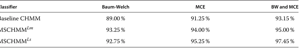
First, we apply the baseline CHMM and the proposed multi-stream CHMM structures to the single stream sequential data where the features are generated from one homogeneous source of information. The MSCHMM architectures treat the single stream sequential data as a double-stream one (each stream is assumed to have 2D observation vectors). In this experiment all models are trained using standard Baum-Welch (for the baseline CHMM), generalized Baum-Welch (for the MSCHMM), standard and generalized MCE/GPD algo-rithms, or a combination of the two (Baum-Welch fol-lowed by MCE/GPD). The results of this experiment are reported in Table 1. As it can be seen, the performance of the proposed MSCHMM structures and the baseline CHMM are comparable for most training methods. This is because when both streams are equally relevant for the entire data, the different streams receive nearly equal weights in all states’ components and the MSCHMM reduces to the baseline CHMM. Figure 1 displays the weights of stream 1 components. As it can be seen, most weights are clustered around 0.5 (maximum weight is less than 0.6 and minimum weight is more than 0.4). Since

Table 1 Classification rates of the different CHMM structures of the single stream data

Classifier Baum-Welch MCE BW and MCE

Baseline CHMM 89.00 % 91.25 % 93.15 %

MSCHMMLm 93.25 % 94.00 % 95.00 %

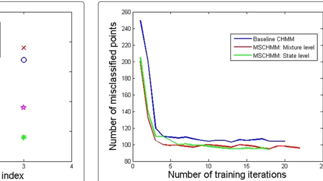
Figure 1Stream 1 relevance weights of the mixture components in all four states, learned by the MSCHMMLmmodel for the single-stream sequential data.

weights of both streams must sum to 1, both weights are equally important for all symbols.

The second experiment involves applying both the base-line CHMM and the proposed MSCHMM to the double stream sequential data where the features are generated from two different streams. In this experiment, the var-ious models are trained using Baum-Welch, MCE, and Baum-Welch followed by MCE training algorithms. First, we note that using stream relevance weights, the gener-alized Baum-Welch and MCE training algorithms con-verge faster and the MCE results in smaller training error. Figure 2 displays the number of misclassified samples ver-sus the number of iterations for the baseline CHMM and the proposed MSCHMM using MCE/GPD training. As it can be seen, learning stream relevance weights causes the error to drop faster. In fact, at each iteration, the clas-sification error for the MSCHMM is lower than that of the baseline CHMM. However, as shown in Table 2, for each iteration, the computational complexity involved in the proposed MSCHMM is about 2.5 times of the baseline CHMM.

The testing results are reported in Table 3. First, we note that all proposed multi-stream CHMMs outperform the baseline CHMM for all training methods. This is because the data set used for this experiment was gen-erated from two streams with different degrees of rele-vance and the baseline CHMM treats both streams equally important. The proposed MSCHMM structures on the other hand, learn the optimal relevance weights for each symbol within each state. The learned weights for stream

1 by the MSCHMMLm are displayed in Figure 3. As it

can be seen, some components are highly relevant (weight close to 1) in some states, while others are completely irrelevant (weights close to 0). The latter ones correspond

Figure 2Number of misclassified samples versus training iteration number for the standard and multistream CHMMs.

to the components where stream 1 features were replaced by noise in the data generation. We should note here that in theory, we assumed that at time t one of the L streams is significantly more relevant than the others in order to derive update equations for all parameters using the Baum-Welch algorithm (refer to Section 3.1). However, in practice, the performance of the algorithm does not break down if this assumption does not hold. For instance, in Figure 1, the weights are equal when all streams are rel-evant while in Figure 3 the weights are different but not binary.

In Table 3, we also compare our approach to the two state of the art MSCHMM that were discussed in Section 2.2. The proposed multi-stream CHMMs out-perform both of these methods. This is mainly due to the fact that the parameters of the proposed MSCHMM structures allow for a simultaneous update for both Baum-Welch and MCE/GPD training. However, for the

MSCHMMG, the parameters learned separately by two

different algorithms and two different objective functions. From Table 3, we also notice that using the general-ized Baum-Welch followed by the MCE to learn the model parameters is a better strategy. This is consistent with what has been reported for the baseline HMM [18].

4.2 Application to landmine detection

4.2.1 Data collection

Figure 3Stream 1 relevance weights of the mixture components in all four states learned by theMSCHMMLmmodel for the double-stream sequential data.

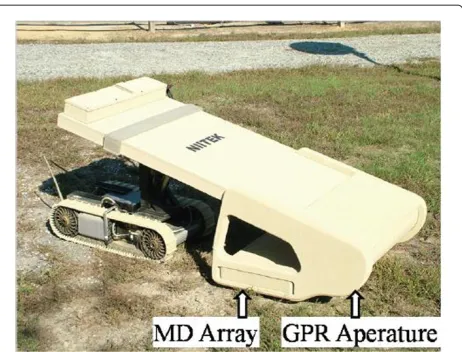
is used in our experiments. The GPR sensor [31] col-lects 24 channels of data. Adjacent channels are spaced approximately 5 cm apart in the cross-track direction, and sequences (or scans) are taken at approximately 1 cen-timeter down-track intervals. The system uses a V-dipole antenna that generates a wide-band pulse ranging from 200 MHz to 7 GHz. Each A-scan, that is, the measured waveform collected in one channel at one down-track position, contains 516 time samples at which the GPR signal return is recorded. We model an entire collection of input data as a 3D matrix of sample values, S(z,x,y); z=1,. . ., 516;x=1,. . ., 24;y=1,. . .,T, whereTis the total number of collected scans, and the indicesz,x, and yrepresent depth, cross-track position, and down-track positions, respectively.

The autonomous mine detection system (shown in Figure 4) was used to acquire large collections of GPR data from two geographically distinct test sites in the east-ern U.S. with natural soil. The two sites are partitioned into grids with known mine locations. Twenty eight dis-tinct mine types that can be classified into four categories: anti-tank metal (ATM), anti-tank with low metal content (ATLM), anti-personal metal (APM), and anti-personal with low metal content (APLM) were used. All targets were buried up to 5 inches deep. Multiple data collections were performed at each site resulting in a large and diverse collection of signatures. In addition to mines, clutter sig-natures were used to test the robustness of the detectors. Clutter arises from two different processes. One type

Figure 4NIITEK autonomous mine detection system.

of clutter is emplaced and surveyed. Objects used for this clutter can be classified into two categories: high metal clutter (HMC) and non-metal clutter (NMC). High metal clutter such as steel scraps, bolts, soft-drink cans, was emplaced and surveyed in an effort to test the robust-ness of the detection algorithms. Non-metal clutter such as concrete blocks and wood blocks was emplaced and surveyed in an effort to test the robustness of the GPR based detection algorithms. The other type of clutter, referred to as blank, is caused by disturbing the soil.

For our experiment, we use a subset of the data collec-tion that includes 600 mine and 600 clutter signatures. The raw GPR data are first preprocessed to enhance the mine signatures for detection. We identify the location of the ground bounce as the signal’s peak and align the multiple signals with respect to their peaks. This align-ment is necessary because the mounted system cannot maintain the radar antenna at a fixed distance above the ground. Since the system is looking for buried objects, the early time samples of each signal, up to few samples beyond the ground bounce are discarded so that only data corresponding to regions below the ground surface are processed.

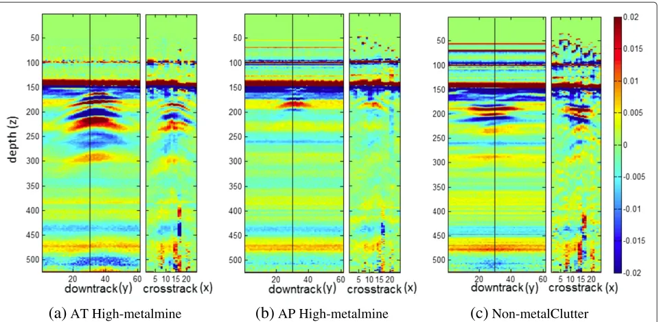
Figure 5 displays several preprocessed B-scans

(sequences of A-scans) both down-track (formed from a time sequence of A-scans from a single sensor channel) and cross-track (formed from each channels response in a single sample) at the position indicated by a line in the down-track. The objects scanned are (a) a high-metal

Table 2 CPU time per iteration for the MCE/GPD training

MCE/GPD Baseline CHMM MSCHMMLm MSCHMMLs

Table 3 Performance of the different CHMM structures on the multi-stream data

Classifier Baum-Welch MCE BW and MCE

Baseline CHMM 63.25 % 65.75 % 68.85 %

MSCHMMLm 70.35 % 72.75 % 79.65 %

MSCHMMLs 71.65 % 71.25 % 80.00 %

MSCHMMGM _{- - 70.65 %}

MSCHMMGS _{- - 72.00 %}

content tank mine, (b) a high-metal content anti-personnel mine, and (c) a wood block. The reflections between depths 50 and 125 in these figures are the artifact of preprocessing and data alignment. The strong reflec-tions between cross-track scans 15 and 20 are due to Electromagnetic interference (or EMI). The preprocess-ing artifacts and the EMI can add considerable amounts of noise to the signatures and make the detection problem more difficult.

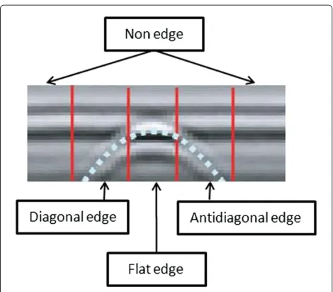
4.2.2 Feature extraction

As it can be seen in Figure 6, landmines (and other buried objects) appear in time domain GPR as hyper-bolic shapes (corrupted by noise), usually preceded and followed by a background area. Thus, the feature repre-sentation adopted by the HMM is based on the degree to which edges occur in the diagonal and antidiagonal

directions, and the features are extracted to accentuate these edges.

Each alarm has over 516 depth values, however, the mine signature is not expected to cover all the depth val-ues. Typically, depending on the mine type and burial depth, the mine signature may extend over 40–200 depth values, i.e., it may cover no more than 10% of the extracted data cube. For example, in Figure 5b, the signature essen-tially extends from depth index 170 to depth index 200. There is a little or no evidence that a mine is present in depth bins above or below this region. Thus, extracting one global feature from the alarm may not discriminate between mine and clutter signatures effectively. To avoid this limitation, we extract the features from a small win-dow withW_d = 45 depth values. Since the ground truth for the depth value (zs) is not provided, we visually inspect

all training mine signatures and estimate this value. For

(a)

(b)

(c)