Object Recognition System-on-Chip Using the Support Vector Machines

(1)

Object Recognition System-on-Chip Using

the Support Vector Machines

Roberto Reyna-Rojas

Laboratory for Analysis and Architecture of Systems (LAAS), CNRS, 7 avenue du Colonel Roche, 31077 Toulouse Cedex 4, France Email:[email protected]

Dominique Houzet

The Rennes Institute of Electronics and Telecommunications (IETR) (UMR CNRS 6164), INSA, 20 avenue des Buttes de Co¨esmes, 35053 Rennes Cedex, France

Email:[email protected]

Daniela Dragomirescu

Laboratory for Analysis and Architecture of Systems (LAAS), CNRS, 7 avenue du Colonel Roche, 31077 Toulouse Cedex 4, France Email:[email protected]

Florent Carlier

Salim Ouadjaout

Received 16 September 2003; Revised 6 June 2004

The first aim of this work is to propose the design of a system-on-chip (SoC) platform dedicated to digital image and signal processing, which is tuned to implement eﬃciently multiply-and-accumulate (MAC) vector/matrix operations. The second aim of this work is to implement a recent promising neural network method, namely, the support vector machine (SVM) used for real-time object recognition, in order to build a vision machine. With such a reconfigurable and programmable SoC platform, it is possible to implement any SVM function dedicated to any object recognition problem. The final aim is to obtain an automatic reconfiguration of the SoC platform, based on the results of the learning phase on an objects’ database, which makes it possible to recognize practically any object without manual programming. Recognition can be of any kind that is from image to signal data. Such a system is a general-purpose automatic classifier. Many applications can be considered as a classification problem, but are usually treated specifically in order to optimize the cost of the implemented solution. The cost of our approach is more important than a dedicated one, but in a near future, hundreds of millions of gates will be common and aﬀordable compared to the design cost. What we are proposing here is a general-purpose classification neural network implemented on a reconfigurable SoC platform. The first version presented here is limited in size and thus in object recognition performances, but can be easily upgraded according to technology improvements.

Keywords and phrases:parallel architecture, pattern recognition, support vector machines, hardware design language,

systems-on-programmable-chip and system-on-chip platforms.

1. INTRODUCTION

This work relates to machine vision but is considered un-der the angle of the hardware design and integration. This work will be centered on specific signal processing circuits. We have chosen the SVM neural network algorithm as our data classification algorithm.

(2)

to use them when the design time is shortened as it is the case with time-to-market constraints. The neural networks by themselves represent a significant research subject in the sci-entific and technological world since a few tens of years. The-oretical bases, performances, architectures, applications, and hardware implementations are some of the studied axis [1].

A machine-vision design relates also to the hardware part of a system. For some particular applications, hardware de-sign goes from the study and the dede-sign of image sensors and optics to computing units. This work is rather centered on the computing units dedicated to application algorithms, using a standard camera for image acquisition. In commer-cial systems, we frequently find architectures using tradi-tional processors, which provide the necessary performances to applications. We also can find architectures with special-ized digital signal processing circuits (DSP), which have suit-able arithmetic units for the necessary precision. Neverthe-less, the regularity of image processing and neural network algorithms cannot be completely exploited by these types of architectures. Parallel architectures are best adapted for hard-ware implementation of vision systems and neural calcula-tions due to their ability to exploit the parallel nature of al-gorithms.

The growing scale of integration has allowed designers to include in the same chip several parts of a system and even the entire system. Systems-on-chip (SoC) is one of the lat-est ideas in system integration. Circuits cannot be designed in a classical way because they are more complex and diﬀ er-ent functions (subsystems) are being integrated. Technology allows more flexible architectures: a larger number of inte-grated gates, less power consumption, higher speeds, bigger and faster integrated memories, processors cores, communi-cations interfaces, and so forth. Object recognition system-on-chip is a natural perspective in the machine perception domain.

InSection 2of this paper, we present the basic idea of the SVM, in particular for classification. InSection 3, we explain the algorithm complexity and the software performances of the SVM method. We briefly present neural architectures in Section 5and some application results inSection 6. In Sec-tions 7and8, we will give the details of our proposed ar-chitecture of the SoC platform solution and we will end our paper with the conclusion and perspectives.

2. THE SUPPORT VECTOR MACHINES

Twenty years ago, the neural networks knew a very signifi-cant importance in scientific and engineering worlds. Nowa-days, industrial products are oﬀered on the market with real success even if we do not have the associated physical model within the automation or the diagnosis. It is necessary to consider the neural networks as a tool for building an em-pirical model with what that supposes of inaccuracy and risk for the application. The theory of the statistical learning be-came more interesting with new results in generalization and with the proposal of the SVM model. Vapnik in the AT&T Bell laboratories proposed the theory of the statistical

learn-F

z1

z2

z3

x1

x2

R2 R3

Φ:R2_→_R3

(x1,x2)→(z1,z2,z3) :=x21,

√ 2x1x2,x22

Figure1: Kernel functions are used to transform the input space into feature space where the optimal hyperplane is constructed.

ing [2,3]. We will very briefly present this theory in order to introduce the generalization function. The details of the theory can be consulted in [2].

The theory of the SVM

The support vector machine model is the most recent propo-sition on neural network structures. This model is based on the statistical learning theory. The support vector machine model consists in a transformation of the input vectorsXin a space of higher dimension Z through a nonlinear trans-formation, selected a priori. It is in this new space Z that we can build an optimal hyperplane [2]. For the particular case of pattern recognition, the SVMs make a distinction of two classes by finding a decision surface constructed from certain points of the entire learning database, called support vectors [4].

Vapnik proposes a representation of an SVM in the form of one-hidden-layer neural network whose number of cells is equal to the number of “support vectors,” and not to the dimension of the space of the internal representations, as we could have supposed it initially. In this manner, the number of neurons is obtained in an automatic way with the reso-lution of a quadratic problem. The support vectors are the input vectorsxifor which equalityyi(w0xi+b0)=1 holds. Concretely, they are the closest points to the optimal hyper-plane. For all other examples, there is thus a factor α = 0 that eliminates them from the solution. We thus know that the decision function is calculated from the examples that are on the margin. In the nonlinear case, it is enough to re-place the scalar products (x·xi) by kernelsk(x,xi). The ker-nel functions were proposed to build nonlinear algorithms from linear algorithms by calculating the inner product not in the input space but in the feature space. Figure 1shows this transformation.

(3)

a solution, for diﬀerent databases, with the minimum num-ber of support vectors. In terms of generalization, we ob-served, particularly in the first application, that the best per-formances were also obtained with the polynomial kernel.

3. COMPLEXITY AND PERFORMANCES

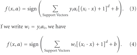
The general equation of the SVM generalization function for classification is

f(x,α)=sign 



Support Vectors

yiαikxi,x+b  _, ₍₁₎

where

(i) yiαi=wiare the network weights, (ii) xiare the support vectors of the solution, (iii) bis the threshold of the function, (iv) k(x,xi) is the kernel function.

As we can see, the solution is the sign of the sum, which is the generalization function for a two-class classification.

In our case, the kernel function is the polynomial func-tion of degreed:

k(x,y)=(x·y+c)d. (2)

The principal parameter of the polynomial kernel func-tion is the polynomial degree. We take as a priori choice a polynomial of degree 2 (a higher degree implied the use of wider data buses in the hardware implementation).

3.1. Complexity

We suppose that the image size istm×tmand thattb×tbis the detection window size.t2

bis thus the number of pixels to be processed by the window of classification. Here we con-sider a decision function of SVM with a polynomial kernel of degreed:

f(x,α)=sign 



Support Vectors

yiαixi·x+ 1 d+b  _. (3)

If we writewi=yiαi, we have

f(x,α)=sign 



Support Vectors

wixi·x+ 1 d+b  _. (4)

To make the classification of all the windows of pixels of one 512×512 image, with no sweeping, and an 8×8 de-tection window, we have 64×64 (tm/tb)2windows to pro-cess. Each window (or input vector) requires t2_b operations (operation=multiplication + addition) for the scalar prod-uct of the kernel function (x·xi) anddmultiplications for power operation, which we also consider as one operation for simplicity. We have then

t2_b+d+ 1 operations per support vector. (5)

Table1: Summary of the algorithm complexity.

Algorithm Number of operations

SVM N×t2

m

SVM sweeping window (tb/ p)2×N×t2m

Convolution M2_×_t2

m

The additional operation is due to the multiplication be-tween the weightwiand the result of the polynomial and the addition of the thresholdb. LetNbe the number of support vectors obtained during learning; we will then have

N×(t2_b+d+ 1) operations per block. (6)

For (tm/tb)2windows per image, we obtain

N×(t2_b+d+ 1)×

tm

tb

2

operations per image. (7)

By making a simplification and knowing that in general, t2_bd+ 1, we thus haveN×t2

moperations per image. That means that the number of operations to be calcu-lated depends on the image size and on the number of sup-port vectors. The size of the window thus does not have a sig-nificant influence on the complexity of the algorithm. Nev-ertheless, this size will represent a fundamental factor during the material implementation because it will be used to di-mension part of the circuit.

Now, if we use a sweeping classification window over the image, we will classify pixels several times. In this case, there will be more windows to analyze per image: (tm/ p)2_{, where} pis the number of sweeping pixels (can also be seen as the classification resolution). For example, for p = 2, we move in the image with a step of 2 pixels at a time, horizontally and vertically. We then get

N×(t2

b+d+ 1)×

tm

p 2

≈

tb

p 2

×N×t2 m

operations per image.

(8)

In the case of an 8×8 detection window and a sweeping step of 2 pixels, we will make 16 times more calculations than without sweeping. The advantage of using sweeping would be to increase the image sampling and to classify several times each pixel or window of pixels and thus to obtain a more robust decision, and also to increase at the same time the localization precision. The complexity for a traditional im-age processing algorithm like filtering by a convolution direct method depends on the size of the convolution mask (M×M for example) and on the size of the processed image, there-fore the number of operations is given by

M2×t2moperations by image. (9)

(4)

Table2: Execution times for diferent image sizes: 16×16 window size, 88 support vectors.

Image size Execution time Execution time_{Sweeping window}

Estimated Measured Estimated Measured 128×128 0.7 s 0.6 s 2.2 s 2.7 s 256×256 2.5 s 2.7 s 9.2 s 10.8 s 512×512 10.2 s 11.0 s 37.0 s 43.9 s

the convolution mask is only the first step to solve the prob-lem of object detection and localization.

In general, if we use a classical method for object recog-nition, the complexity of the system will be the addition of the complexity of each subsystem. It will also depend on dif-ferent parameters of the processed image, for example, edges density, line density, and the ratio between the object and the image size. For the SVM method, the complexity depends only on a priori chosen parameters.

3.2. Performances

We carried out some measurements of execution times. As we have shown, the number of operations and the comput-ing time increase proportionally to the number of support vectors. We thus found the main disadvantage of the support vector machine method: the number of support vectors. This number is automatically obtained during learning; we can-not control this parameter without modifying the general-ization performances.

These measurements of execution times were made on a Sun Microsystems Ultra 5 Workstation.

For the estimation of the computing time, we obtained that a multiplication-addition operation is executed in 470 nanoseconds. We obtained this time from a program carry-ing out a loop of 106_{iterations. In this loop as in the} soft-ware implementation of the function of generalization of the SVM, we used the mathematical function pow(·). Estimated times are slightly larger than measured times. This is due to the use of the indices in the estimation program.Table 2 shows some results.

3.3. Learning performances

The learning algorithm uses a decomposition method to in-crease the learning performance and to reduce the necessary resources of the machine on which we execute the learn-ing algorithm, in particular, memory resources. This algo-rithm calls the generalization function and supposes that we can define a working set (vectors or examples) B such as |B| ≤L(Lis equal to the number of examples or vectors of all the learning database, and|B|the number ofBelements). This set is suﬃciently large to contain all the support vectors (αi>0), but suﬃciently small so that the hardware platform (PC, workstation, etc.) can handle and optimize them by us-ing the quadratic optimization algorithm.

The decomposition technique can be written in the fol-lowing manner.

1400 1200 1000 800 600 400 200 0

Ti

m

e

(s

)

0 100 200 300 400 500 600 700 800 Size of the work subsetB

Total execution time Optimization subroutine Generalization subroutine

Figure 2: Execution time of the learning program and the opti-mization and generalization subroutines of the SVM method, ob-tained by using a database of 4096 examples of dimension 64.

(1) Choose in a random way|B|points of the database. (2) Resolve the subproblem defined by the elements inB. (3) Repeat the three steps while there exists a j ∈Nsuch

asg(xj)·yj <1 (which corresponds to a bad classifi-cation), where

gxj=

l

p=1

ypαpKxj,xp

+b. (10)

The algorithm, at each iteration, improves the objective (optimization) function and is not, in this sense, recursive. Since the objective function is limited, the algorithm con-verges towards the optimal solution in a finite number of it-erations [5].

The function g(xj) is in fact the SVM generalization function; and for instance, if we are able to reduce two orders of magnitude, the execution time of this part of the algorithm will improve the learning performances and we could have a real-time learning algorithm.

We can observe the experimental results of the execution time of the learning algorithm according to the size of the working subsetBinFigure 2. The learning process is clearly accelerated with this decomposition method. According to these simulation results, for a real-time learning system and for subsets of average sizes, it would be necessary to increase the performances of the execution of the quadratic optimiza-tion algorithm. We can also observe inFigure 2that the exe-cution time of the SVM generalization function is practically constant, which is approximately 100 seconds. This is be-cause the calculation ofg(xj) is made for alljof the database and thus does not depend onB. ForBlower than 200, the execution time of the learning algorithm is practically domi-nated by the generalization subroutine.

(5)

the results on one of the three tested applications and then we are going to detail the architecture at diﬀerent levels.

4. APPLICATIONS

The excellent performances of the SVM for classification problems were very attractive from the beginning of their proposal. This is true especially if we consider that the method can be applied directly on pixel values, it does not need to take into account any other a priori problem knowl-edge, and “a permutation of the images by a fixed transfor-mation does not modify the SVM classifier performances” [6].

The performance analysis of the SVM methods on databases used as “benchmarks” by the scientific community was already reported in literature [2,7]. Other evaluations were made on synthetic databases [8]. The principal inter-est of our contribution is to study this method for real-life applications (matrix barcodes detection, face detection in an automobile cockpit, and the white lines detection). We have found that the SVM method makes, possible to build very powerful classifiers (polynomial, RBF, or perceptron).

4.1. Detection and localization of matrix barcodes Barcodes are essential as a product identification, either dur-ing manufacturdur-ing or durdur-ing marketdur-ing. The market require-ments made very important the fine resolution of questions like reading robustness under very diverse conditions. The eﬀectiveness of barcodes is so interesting that the vendors would wish to be able to put more information on them. A linear barcode, for example EAN13 code, can code 11 char-acters (numerical 0–9); this code is generally used like refer-ence for a product index. The aim of matrix barcodes is to be able to code more than 2000 alphanumeric characters, and to thus be able to have product information like their price and their principal features. That supposes to evolve from a one-dimensional code to a dimensional code; and two-dimensional codes suppose image processing and recogni-tion.

This study was made with the collaboration of Intermec Company. Intermec provided a base of 78 images with dif-ferent types of matrix barcodes and various image sizes. The study was based on the DataMatrix code. We have also shown results of generalization on other types of codes. Each pixel value is coded on eight bits, that it, in 256 gray levels from 0 to 255.

The images show different scenarios like projective defor-mations, different image backgrounds, different scales, and so forth. For this application, we find the object by segment-ing the image and not by findsegment-ing directly the whole object, that is, we benefit from the texture regularity of matrix bar-codes to locate them. In [9], the author proposes, for the lo-calization and the automatic reading of matrix barcodes, to use the texture to validate the different zones found by the lo-calization algorithm. The objective for this first application is thus to learn texture from a matrix barcode DataMatrix and to make a localization of these codes in new images through image segmentation.

Class−1

Class +1

Figure3: Definition of the two classes for matrix barcodes detec-tion.

Table3: Number of support vectors found during learning for dif-ferent kernels and values of parameter C.

Kernel Degree Value of C

10 200 500 5000

Linear — 491 547 620 1320

Polynomial 2 316 310 321 320

Polynomial 3 333 343 325 311

Polynomial 4 341 310 311 311

RBF 2 385 333 312 304

Databases creation is a delicate task for the methods that use supervised learning algorithms. The solution of the neu-ral network will depend exclusively on the examples of the learning database. Since the SVM method is also based on learning from examples, a given “optimal” learning database provides an “optimal” solution.

In this application, we feed the learning algorithm with examples of the “positive” parts of the image (a matrix bar-code), and with other textures (text, images, etc.) as “nega-tive” examples. Two classes are thus defined (seeFigure 3): a block of pixels with the texture of the matrix barcode (class +1) and a block of pixels with a diﬀerent texture (class−1). Two detection window sizes were tested: 8×8 pixels and 16×16 pixels.

We present the learning results over one database and the respective result in generalization. The first database was cre-ated from the image shown inFigure 3. InTable 3, we show learning results with a database of 4096 input vectors of di-mension 64 (8×8 pixels) with 240 positive examples. The number of support vectors is indicated inTable 3for differ-ent kernel functions and differdiffer-ent values of the penalization parameter C.

We created a test database from three diﬀerent images. This test database consists of 12 288 examples, including 10% of positive examples. In generalization, we obtained 91.8% of good classifications (positive or negative), 3.8% of no detec-tion (when the example is positive and the result of gener-alization is negative), and 4.2% of false detection (when the example is negative and the result of generalization is posi-tive).

(6)

(a) (b)

(c) (d)

Figure4: Image segmentation results using the SVM as detection system. The window size is 8×8 pixels. A postprocessing algorithm is used in order to erase the bad classifications of the SVM.

having a relatively small percentage of false alarms compared to the number of no detection led us to define a postprocess-ing module based on a morphological processpostprocess-ing for this par-ticular application. In the images ofFigure 4, we show some qualitative results of detection, that is, we show two examples of the output binary images.

We seek to use the best solution with a minimal num-ber of support vectors. These results were obtained with the second-degree polynomial kernel function solution and with the penalization parameter C =200. The first image shows the result of the test since the learning database was created using this image. More detailed information can be found in [10].

5. PARALLEL NEURAL ARCHITECTURES

The regularity of image processing and neural network al-gorithms encourages the use of parallel VLSI circuits. Paral-lelism is an intrinsic notion of the neural networks, which are regarded as massively parallel systems [11]. In spite of the enormous computing power obtained with new se-quential processors, it is possible that these types of pro-cessors are not suﬃcient for real-time applications. There are some solutions with neural networks, which use classi-cal sequential processors, for example, the opticlassi-cal charac-ter recognition (OCR) algorithms, whose performances are acceptable for applications that do not require a real-time operation.

A significant number of analog implementations were proposed, exploiting the biological origin of neural net-works, which illustrates the use of individual simple cells but interconnected by a network and functioning in a massively parallel way. In the particular case of the integrated artifi-cial retinas, the use of analog circuits is a choice impossible to avoid, because we want to be able to bring processing as near as possible to the photosensitive circuit and to be able to manage the interconnections more easily (each pixel in-teracts with its closer neighbors) [12,13].

Many neural implementations in numerical integrated circuits have been proposed. The finality of these circuits is to be used within traditional workstations like neural copro-cessors, in acquisition and signal processing cards, in order to make more intelligent sensors, or to be used as specialized parallel-processing machines. They are generally dedicated to a single neural model, and all do not propose a learning inte-grated procedure [14]. There are thus several types of neural systems.

(1) Application-specific architectures implement a mod-el, a topology, and a set of weights, mostly by analog means.

(2) Problem-specific architectures implement a model and a given topology; the weights of the network are pro-grammable. The learning is done most of the time oﬀ-line.

(3) With algorithm-specific architectures, the model is selected a priori. Topology can be modified, and the learn-ing is carried out by the system itself.

(4) Neural processor architectures are also called multi-model accelerators. They are much closer to a generic pro-cessor [14,15].

(7)

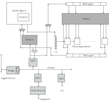
CAN/CNA(10)

Analog I/O

(11)

FIFO _FIFO

Digital I/O(12) Bridge FI_FO

OCB(5) FIFO

RAM(3)

(7)

Shift reg(9) Processing units(6)

Shift reg(8)

RAM(4) Cache(2)

LEON-light(1)

Figure5: SoC platform architecture.

preloaded coeﬃcients and accumulates the result from the macrocells in the column above it. The columns simulta-neously calculate the results in one processor cycle. For 8-bit data and coeﬃcients, the vector coprocessor performs 24 MAC (multiply-accumulate) operations with 21-bit results in one processor cycle. The number of MAC operations de-pends on the length and number of words packed into a 64-bit block. The engine’s configuration can change dynami-cally during calculations. An application can start with max-imum precision and minmax-imum performance and dynami-cally increases the performance by reducing the data-word lengths.

6. THE OBJECT RECOGNITION SYSTEM

If we take the classical and simplified architecture of an object recognition system, we have the following modules: image sensor, detection, localization, and diagnosis. For our imple-mentation, we propose a PC-based recognition system, and use a standard camera as an image sensor. Therefore, it is the detection module that we will hardware-implement using the SVM as its core. In order to be able to integrate the detection module in the PC-based system, we will use the PCI inter-face.

7. THE SOC PLATFORM ARCHITECTURE

A particular SoC category concerns the SoC platforms [19], an emerging technology whose main purpose is to provide a reusable silicon platform for many applications, either for several versions of a single application or even for several diﬀerent applications in the same field. This is due to the growing design and fabrication costs of ASICs, which thus impose large amounts of chips. The only solution is to have more general reusable chips. The Xilinx VirtexPro II can be considered as a general-purpose SoC platform, which asso-ciates dedicated blocks such as PowerPC processors, RAM and multipliers, and a classic FPGA part that can be dynam-ically reconfigured.

(8)

@start1 Size1 @start2 Size2 @Dest. Precision OP1 OP2 Broad Accum.

Figure6: Configuration instruction register.

OP1: ALU X ALU X

OP2: ALU ALU

Figure7: Multiprecision processing unit.

to communicate directly from its cache memory (2) to the dual-ported RAM (3) used to store LEON2’s binary code and data. A second data RAM (4) is accessible in the memory address space of both the LEON2 processor and the exter-nal I/O subsystem (5), which is here a simple on-chip bus with its wrappers (light-gray boxes). This dual-ported RAM is the storage unit of the CP vector/matrix unit (6) which per-forms ALU/MAC operations loops on vector/matrix fixed-point data from the RAM, according to the instruction reg-ister (7) which provides the configuration of the processing units. This register is detailed inFigure 6. The ALU allows any kind of operations to be executed, leading to a richer in-struction set than the simple MAC operations of most similar approaches such as the NeuroMatrix chip [18].

This is a double register operating in ping-pong mode. This register is reconfigured for each new matrix operation. The configuration that is provided to the vector processing unit is the size, step, and addresses of the loops, the preci-sion of data, and the operations performed with or without accumulation.

Here it is an example of vector/matrix operation with ac-cumulation.

The (8) and (9) registers are used to shift input and out-put data in and out of the vector RAM. These registers can also broadcast input and output data in the case of vec-tor/matrix operations to be treated as matrix/matrix oper-ations.

The multiprecision unit is presented onFigure 7. This is a version with only two diﬀerent input precisions (8-bit and 16-bit) in order to simplify the presentation. The first OP1 operator is either an 8×8 multiply or an 8-bit ALU. The 16-bit result can be accumulated with the 32-bit OP2 opera-tor. The two 8-bit multiply operators (OP1) can also be com-bined to perform a 16-bit multiply in two clock cycles, using

the accumulation operator (OP2) to perform the two addi-tions. A 16-bit MAC is thus performed in four clock cycles, that is, two for the four multiply operations, one for the last addition of the 16-bit multiply results, and one for the final accumulation. The accumulation is pipelined with the pre-ceding operation, which is thus treated every clock cycle for an 8-bit MAC, every three cycles for a 16-bit MAC, and every five cycles for a 32-bit MAC, that is, everyN+ 2 cycles withN being the number of bytes of data precision. The main limita-tion of our proposed architecture is the vector data precision which must be a multiple of 8 bits, which however is often the case in image processing. The counterpart is the lower complexity of the logic which leads to higher clock frequen-cies, compared to the NeuroMatrix solution which is a 1-bit multiple with a lower clock frequency.

The last part of the system is the I/O subsystem, which has to feed the processor with data. The OCB is used as the central communication subsystem between the proces-sor/coprocessor and the external analog (10) and digital (12) ports. Other components can also be integrated on the OCB (11), like other processor/coprocessor couples, in order to build a complex system. A single large coprocessor with many processing units would be diﬃcult to manage due to the lim-ited available data and instruction parallelism as well as the long distances between units which would aﬀect their com-munications and the clock frequency. Here is Algorithm 1 an example of configuration obtained from the original and adapted C SVM source codes of Algorithms2and3. The co-processor here executes only the two internal loops. These internal loops are packed in a function.

(9)

int CP Recognition(int nb sensors, int nb supports) {intk,j;

for(j=0;j <nb supports;j+ +) for(k=0;k <nb sensors,k+ +)

oo[j]+=support vectors[nb sensors∗j+k]∗sample[k];}

Support vector nb Supports sample nb sensors oo 8 + x no acc.

Algorithm1: CP Recognition(·) function and equivalent configuration.

/** RECONNAISSANCE ******************************************************/ /**************************************************************************/ void

recognition(sample, nb samples, nb sensors, std, support vectors, support weights, support threshold, nb supports, kernel, classe, gausse, var thresh)

int *sample; int nb samples;

int nb sensors; float std;

int *support vectors; float *support weights; float support threshold; int nb supports;

char *kernel; int *classe;

double var thresh; {

double out; double oo; int i,j,k; struct timeb debut,final; FILE *fichier; for(i=0;i <nb samples;i+ +){

out=0.0;

for(j=0;j <nb supports;j+ +){ oo=0.0;

if (kernel[0]==‘p){

for(k=0;k <nb sensors;k+ +)

oo +=(support vectors [nb sensors *j+k]* sample[nb sensors *i+k]); out +=support weights [j]* pow (oo +1.0 std);

} }

OUT +=support threshold; if(out>=var thresh)

classe [i]=1; else

classe [i]= −1; }

}

Algorithm2: Original C-code of the SVM generalization function. The part of the code that is executed on the coprocessor is underlined.

for (i=0;i <nb samples;i+ +){out=0; for (j=0;j <nb supports;j+ +) oo [j]=0;

CP Recognition(nb sensors,nb supports); // non blocking Acquisition(sample); // non blocking

Sync(); // blocking

for (j=0;j <nb supports;j+ +) out +=support weights [j]∗pow(oo[j] + 1); out +=support threshold;

if (out>=var thread) classe [i]=1; else classe [i]=0;}

(10)

For (J=start2;J <size2;J+=step2){ For (I=start1;I <size1;I+=step1){

Res[J]=Res[J] op2 (RAM1[I] op1 RAM2[I]);} }

Algorithm4: General parallel loop pattern.

based on a static compile-time generation of configurations, which is most of the time suﬃcient and as easy to program as our solution, but dynamicity becomes more and more im-portant. This is particularly important when the reconfigu-ration needs to be dependent on the previous results of a processing, in a nonpredictable way. The heart of our learn-ing procedure is based on the classification procedure, which is evaluated here. The dynamic nature of the parameters is used here in the learning phase, which calculates the inter-esting support vectors, their number, and their size accord-ing to the quality of the classification. These results can be reinjected in the classifier treatment in order to size the fi-nal classifier parameters. Thus, this nonsupervised approach leads to an automatic parameterization of the classification treatment. This SVM solution, which is optimal in terms of database classification, can thus be used as an automatic so-lution to many treatments, which can be adapted and solved by means of classification. This kind of approach is only pos-sible if a large-size hardware is available, that is, in a near fu-ture.

This application could be also implemented on the Neu-romatrix chip, but with lower execution time (or higher costs). The scalability of the application, which is linear for matrix operations, can be dealt within two ways. First, when the size of the loops is higher than the size of the coprocessor, a second internal level of loop is performed in the coproces-sor structure by means of RAM address management, that is, with a circular data mapping in the RAM array. Second, when the data size is higher than the RAM size, the treat-ment has to be divided in smaller parts manually at com-pile time, either on the same coprocessor by serialization, or on several diﬀerent coprocessors linked together through the network-on-chip, which is here the PCI-X on-chip bus. A future data cache RAM array architecture is under study in order to mask this limitation to the programmer. Both solu-tions lead to performances or cost impact due to serialization of operations.

8. RESULTS

8.1. The choice on SVM parameters

The retained kernel function of the SVM machine is the poly-nomial, because of the obtained performances and also be-cause its hardware implementation is relatively easier. The principal parameter of the polynomial kernel function is the degree of the polynomial. Although it is possible to make an implementation with a variable polynomial degree, we took as basic choice a polynomial of degree 2 (a higher de-gree would impose the use of wider data buses). Considering that our principal application is the matrix barcodes

detec-Table4: Hardware parameters summary.

Parameters Memory size

Input dimension 256 pixels 32×32 bytes

Input precision 8 bits —

Kernel Polynomial —

Degree 2–4 —

Number of SV 128 128×256 bytes

Weights precision 24 bits 128×3 bytes

Table5: SVM core behavioral specification.

Kernel function Polynomial

Degree of the kernel function 2/3/4

Number of support vectors 128

Input dimension 64 or 256

tion, we took 16×16 pixels as the detection window size for the hardware implementation. This size is not important to the application level.Table 4summarizes the hardware pa-rameters andTable 5the behavioral specification of the SVM classifier.

8.2. The choice of the hardware parameters

We have chosen to implement the SVM classifier on a SoC platform in order to exploit the parallel nature of the SVM algorithm. The active logical blocks and the interconnection buses normally consume the surface of silicon of an ASIC or FPGA circuit. For a few years, interconnection busses became the main consumers of silicon surface, due to the complexity of algorithms and circuits.

Input data. The values of pixels are coded in 256 gray lev-els, therefore all memories with pixel values will be used as a multiple of 8 bits. So each element of the support vectors will correspond to an 8-bit value.

Weight Data. It is the only data whose size is not defined by the specification. It is significant to define its size pre-cisely, in order not to modify the recognition performances significantly. Although the values in the software implemen-tation, are float values, in the hardware implemenimplemen-tation, we use fixed point to avoid the use of the floating-point opera-tors. The results of weights precision analysis were obtained from the same database used for testing the SVM algorithm. We vary the precision (number of bits) of the weights and we obtain the percentage of good detection and of bad classifi-cations, the rest corresponding to false alarms.

(11)

CAN/CNA FPGA _OCB RAM

LEON Light FI

FO

PCI BRIDGE

PCI-X Bus

Vector/Matrix CoProcessor FPGA XC2V3000

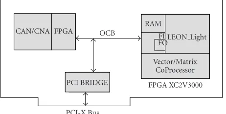
Figure8: FPGA-based prototyping platform.

Table6: VHDL XC2V3000 synthesis summary.

Blocks Size Frequency

32-bit LEON2-light 14% 50 MHz

64-bit OCB interface 6% 133 MHz

64 8-bit coprocessors 60% 166 MHz

LEON2 RAM 32 KB —

Coproc. RAM 128 KB —

fewer neurons than the SVM: this requires less precision for a hardware implementation. And finally, we recall that the hyperplane of separation in the case of the SVM is in a di-mension which is much higher than the input didi-mension, and that the solution is built up using the support vectors. The 32 bits of the processor outputs are suﬃcient to pro-vide the result to the generalization function, which operates on the data weights. The LEON processor performs this last function, which is limited in complexity, sequentially, and in pipeline with the matrix product.

8.3. Prototyping platform

We have designed a general rapid prototyping platform dedicated to SoC emulation. The central board connects a CAN/CNA module with a Xilinx XC2V3000 FPGA and a PCI-X controller. This general-purpose board is presented in Figure 8. A more complex system can be built with several boards on the PCI-X bus, which corresponds to the OCB of our final SoC. We have implemented and validated the pre-sented application on this single board. The synthesis results obtained are presented on Table 6. The vector coprocessor RAM is organized in two 1 KB RAM per processing unit. The peak performances of 10 Giga MAC/s have been reached with this application. As a comparison, the number of gates of our chip is nearly the double compared to the Neuromatrix core. Also, the main vector/matrix product consists of 256∗88 8-bit multiplies, that is, 256∗88/64=352 clock cycles com-pared to the 16∗88=1408 clock cycles with the evaluated Neuromatrix chip. We have thus obtained an eﬃcient solu-tion, easy to program. A large SoC will be studied on CMOS 0.13µm technology ASIC in order to obtain real-time execu-tion with more important applicaexecu-tions.

9. CONCLUSION

Platform-based design (PBD) is the best-validated industrial approach for achieving high reuse in SoC design, and incurs the lowest risk in derivative creation via user programmabil-ity. Although these platforms already exist in some applica-tion domains, their design process is largely ad hoc. Further-more, despite high development costs, such platforms tend to be diﬃcult to program, and very little software support is available. Our proposition attempts to fill this gap. Our proach is to provide a general-purpose neural network ap-plication customized by a learning phase instead of explicit programming which avoid tedious designing eﬀort. Such a solution is only possible with large hardware platforms. We have proposed in this paper a sizeable SoC platform dedi-cated to regular image and signal processing involving ma-trix operations. We have illustrated its implementation ca-pabilities with the SVM neural network application, which performs object recognition of any kind (image or signal). A user-friendly interface is under construction. Also a future ASIC SoC implementation will demonstrate the feasibility of our approach on realistic objects recognition. With such a system, it is possible to obtain an automatic object recog-nition/classification based on a learning phase, which auto-matically configures the recognition engine, and then obtain a real-time toolbox for any object classification.

ACKNOWLEDGMENTS

We thank Intermec for the image databases used to show the performances of the SVM method for a real application. Roberto Reyna-Rojas thanks the Mexican Research Coun-cil for its financial support through the Studentship 111030. This work was supported in part by the Mexican Research Council CONACYT under Student Scholarship 111030.

REFERENCES

[1] C. M. Bishop,Neural Networks for Pattern Recognition, Oxford University Press, Oxford, UK, 1995.

[2] V. N. Vapnik, Statistical Learning Theory, Wiley-Interscience Publication, New York, NY, USA, 1998.

[3] B. E. Boser, I. M. Guyon, and V. N. Vapnik, “A training al-gorithm for optimal margin classifiers,” inProc. 5th ACM Workshop on Computational Learning Theory (COLT ’92), pp. 144–152, Pittsburgh, Pa, USA, July 1992.

[4] C. Burges, A Tutorial on Support Vector Machines for Pat-tern Recognition, Kluwer Academic Publishers, Boston, Mass, USA, 1998.

[5] E. Osuna and F. Girosi, “Reducing the run-time complexity of support vector machines,” inProc. International Conference on Pattern Recognition (ICPR ’98), Brisbane, Australia, August 1998.

[6] Y. LeCun, L. D. Jackel, L. Bottou, et al., “Comparison of learn-ing algorithms for handwritten digit recognition,” inProc. In-ternational Conference on Artificial Neural Networks (ICANN ’95), F. Fogelman-Souli´e and P. Gallinari, Eds., vol. 2, pp. 53– 60, Paris, France, October 1995.

[7] B. Sch¨olkopf, Support vector learning, Ph.D. dissertation, Technical University of Berlin, Berlin, Germany, 1997. [8] V. L. Brailovsky, O. Barzilay, and R. Shahave, “On global,

(12)

machines,”Pattern Recognition Letters, vol. 20, no. 11-13, pp. 1183–1190, 1999.

[9] B. Marcel, Study on the automatic reading of two-dimensional codes by image processing, Ph.D. dissertation, Institut National Polytechnique de Toulouse, Toulouse, France, 1997.

[10] R. Reyna-Rojas, N. Hernandez, D. Esteve, and M. Cattoen, “Segmenting images with support vector machines,” inProc. International Conference on Image Processing (ICIP ’00), vol. 1, pp. 820–823, Vancouver, BC, Canada, September 2000. [11] A. Jain, R. Duin, and J. Mao, “Statistical pattern recognition:

a review,” IEEE Trans. Pattern Anal. Machine Intell., vol. 22, no. 1, pp. 4–37, 2000.

[12] T. Delbr¨uck and C. A. Mead, “Analog VLSI phototransduc-tion by continuous-time, adaptive, logarithmic photorecep-tor circuits,” inVision Chips: Implementing Vision Algorithms with Analog VLSI Circuits, C. Koch and H. Li, Eds., pp. 139– 161, IEEE Computer Society Press, Los Alamitos, Calif, USA, 1994.

[13] L. O. Chua and L. Yang, “Cellular neural networks: applica-tions,” IEEE Trans. Circuits Syst., vol. 35, no. 10, pp. 1273– 1290, 1988.

[14] M. F. Emirian, Study and design of a parallel machine multi-models for the neural networks, Ph.D. thesis, Institut National Polytechnique de Toulouse, Toulouse, France, 1996.

[15] M. Viredaz, Design and analysis of a systolic array for neural computation, Ph.D. thesis, Ecole Polytechnique F´ed´erale de Lausanne, Lausanne, Switzerland, 1994.

[16] P. Clarke, “Siroyan implements clustered DSP architecture,” EE Times, October 2001.

[17] M. Long, “ChipWrights Intros New Visual Signal Processor,” ECN magazine, October 2003.

[18] VLIW/SIMD NeuroMatrix Core, Research Center MODULE, Moscow, Russia.

[19] A. Sangiovanni-Vincentelli and G. Martin, “Platform-based design and software design methodology for embedded sys-tems,”IEEE Des. Test. Comput., vol. 18, no. 6, pp. 23–33, 2001. [20] L. Benini and G. De Micheli, “Networks on chips: a new SoC

paradigm,”IEEE Computer, vol. 35, no. 1, pp. 70–78, 2002. [21] A. Bermak, Sysneuro: un circuit systolique neuronal

mul-tiprécision pour des tâches de classification, Ph.D. thesis, Uni-versité Paul Sabatier de Toulouse, Toulouse, France, 1998. [22] P. Moerland and E. Fiesler, “Neural network adaptations to

hardware implementations,” inHandbook of Neural Com-putation, chapter E1.2, pp. 1–13, Institute of Physics Pub-lishing, Bristol, UK; Oxford University Press, New York, NY, USA, January 1997, IDIAP Research Report IDIAP-RR 97-17.

Roberto Reyna-Rojaswas born in

Tehuan-tepec, Mexico, in 1972. He received the Elec-tronics Engineering degree from the Uni-versidad Aut ´onoma Metropolitana, Mex-ico City, in 1994, and the Computer Sci-ence Engineering degree from ENSEEIHT, Toulouse, France, in 1997. He obtained the Ph.D. degree from the National Institute of Applied Sciences, Toulouse, France, in 2002. He is actually working for the French Space

Agency CNES in VLSI circuits failure analysis, and particularly fail-ures provoked by ESD events. His research interests are in the ar-eas of VLSI design and reliability, development of integrated neural networks, and specific signal processing architectures.

Dominique Houzetreceived the M.S.

de-gree in computer sciences in 1989 from Paul Sabatier University, Toulouse, France, and the Ph.D. degree and HDR degree in com-puter architecture in 1992 and 1999 both from INPT, ENSEEIHT, Toulouse, France. He worked at IRIT Laboratory and EN-SEEIHT Engineering School from 1992 to 2002 as an Assistant Professor and also as a Digital Design Consultant with SME. He

is an Associate Professor in the Department of Telecom, the Na-tional Institute of Applied Sciences, and IETR Laboratory, Rennes, France, since 2002. He has published a number of research papers in the area of parallel computer architecture and SoC design and a book on VHDL principles. His research interests include code-sign and SoC decode-sign methodologies applied to image processing and radiocommunications. He is a Member of the IEEE Computer Society.

Daniela Dragomirescu was born in

Bucharest, Romania, in 1972. She received the Electronics Engineering degree from Bucharest Polytechnic University, Romania, in 1996, and her Ph.D. degree from the National Institute of Applied Sciences, Toulouse, France. She has been an Associate Professor at Toulouse National Institute of Applied Sciences (INSA) since October 2001 and a researcher at Laboratory for

Analysis and Architecture of Systems (LAAS) French National Center for Scientific Research (CNRS). Her research interests are in the area of systems-on-chip and hardware architectures for signal processing.

Florent Carlier received the Ph.D. degree

from the National Institute of Applied Sci-ences, Rennes, France, in 2003, where he specialized in neural networks for commu-nication systems. He has been an IEEE Stu-dent Member. He began an academic career in 2004, as a Lecturer in numerical electron-ics and member of the Department of Infor-matics (LIUM), the University of Maine, Le Mans, France. His research interests include

computer architecture, digital systems, protocol design, and com-puter programming.

Salim Ouadjaoutreceived an M.S. degree in

computer science from the National Insti-tute of Computers (INI), Algeria, in 2000, and an M.S. degree from INP, ENSEEIHT, Toulouse, France, in 2001. He is a Ph.D. candidate in electrical and computer en-gineering at the Institute of Electronics and Telecommunication, Rennes, France. He is also working as a research engineer at M3Systems Inc. He has been an ACM