Objective Speech Quality Measurement Using
Statistical Data Mining
Wei Zha
Power, Acquisition and Telemetry Group, Schlumberger Technology Corporation, 150 Gillingham Lane, MD 1, Sugar Land, TX 77478, USA
Email:[email protected]
Wai-Yip Chan
Department of Electrical & Computer Engineering, Queen’s University, Kingston, ON, Canada K7L 3N6 Email:[email protected]
Received 7 November 2003; Revised 3 September 2004
Measuring speech quality by machines overcomes two major drawbacks of subjective listening tests, their low speed and high cost. Real-time, accurate, and economical objective measurement of speech quality opens up a wide range of applications that cannot be supported with subjective listening tests. In this paper, we propose a statistical data mining approach to design objective speech quality measurement algorithms. A large pool of perceptual distortion features is extracted from the speech signal. We examine using classification and regression trees (CART) and multivariate adaptive regression splines (MARS), separately and jointly, to select the most salient features from the pool, and to construct good estimators of subjective listening quality based on the selected features. We show designs that use perceptually significant features and outperform the state-of-the-art objective measurement algorithm. The designed algorithms are computationally simple, making them suitable for real-time implementation. The pro-posed design method is scalable with the amount of learning data; thus, performance can be improved with more offline or online training.
Keywords and phrases:speech quality, speech perception, mean opinion scores, data mining, classification trees, regression.
1. INTRODUCTION
“Plain old telephone service,” as traditionally provided using dedicated circuit-switched networks, is reliable and econom-ical. A contemporary challenge is to provide high-quality, re-liable, and low-cost voice telephone services over nondedi-cated and heterogeneous networks. Good voice quality is a key factor in garnering customer satisfaction. In a dynamic network, voice quality can be maintained through a combi-nation of measures: design planning, online quality monitor-ing, and call control. Underlying these measures is the need to measure user opinion of voice quality. Traditionally, user opinion is measured offline using subjective listening tests. Such tests are slow and costly. In contrast, machine compu-tation (“objective measurement”), which involves no human subjects, provides a rapid and economical means to estimate user opinion. Objective measurement enables network ser-vice providers to rapidly provision new network connectiv-ity and voice services. Online objective measurement is the only viable means of measuring voice quality, for the pur-pose of real-time call monitoring and control, on a network-wide scale. Other applications of voice quality measurement
include evaluation of disordered speech [1] and synthesized speech [2].
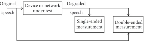
Algorithms for objective measurement of speech qual-ity can be divided into two types: single-ended and double-ended (seeFigure 1). Double-ended algorithms need to in-put both the original (“clean”) and degraded speech signals, whereas single-ended algorithms need only to input the de-graded speech signal. Single-ended algorithms can be used for “passive” monitoring, that is, nonintrusively tapping into a voice connection. Double-ended algorithms are sometimes called “intrusive” because a voice signal known to the algo-rithm has to be injected into the transmit end. Neverthe-less, Conway in [3] proposes a method that employs double-ended algorithms without intruding on an ongoing call. The method is based on measuring packet degradations at the re-ceive end. The measured degradations are applied to atypical
speech signal to produce a degraded signal. A double-ended algorithm is used to map the speech signal and degraded sig-nal to speech quality.
Original speech
Device or network under test
Degraded speech
Single-ended
measurement Double-endedmeasurement
Figure1: Single-ended and double-ended speech quality measure-ments.
obtained from subjective tests as accuracy benchmarks. The
mean opinion score(MOS) [4], obtained by averaging the ab-solute categorical ratings (ACRs) produced by a group of lis-teners, is the most commonly used measure of user opinion. Subjective listening tests are generally performed with a lim-ited number of listeners, so that the MOS varies with the lis-tener sample and its size. In such a case, the degree of accu-racy of objective scores can be assessed up to the degree of accuracy of the subjective scores used as benchmarks.
The International Telecommunications Union (ITU) standard [5, P.862], also called Perceptual Evaluation of Speech Quality (PESQ), is a double-ended algorithm that ex-emplifies the “state-of-the-art.” An ITU standard for single-ended quality measurement [6, P.563] has recently reached a “prepublished” status. Objective measurement has the ad-vantage of being consistent. While subjective tests can be used to estimate the MOS very accurately by using a large listening panel, objective measurement can provide a more accurate MOS estimate than a small listener panel (see [7] for a simple model of measurement variance). Hence, objec-tive measurement, which can be automated and performed in real time, provides a very attractive alternative to subjec-tive tests.
The process of human judgment of speech quality can be modeled in two parts. The first part, auditory perception, en-tails transduction of the received speech acoustic signal into auditory nerve excitations. Auditory models are well stud-ied in the literature [8] and have been applied to the de-sign of PESQ and other objective measurement algorithms [9,10,11]. Essential elements of auditory processing include bark-scale frequency warping and spectral power to sub-jective loudness conversion. The second part of the human judgment process entails cognitive processing in the brain, where compact features related to normative and anomalous behaviors in speech are extracted from auditory excitations and integrated to form a final impression of the perceived speech signal quality. Cognitive models of speech distortions are less well developed. Nevertheless, for the goal of accurate prediction of subjective opinion of speech quality, anthro-pomorphic modeling of cognitive processing is not strictly necessary.
In place of cognitive modeling, we pursue a statisti-cal data mining approach to design novel double-ended al-gorithms. The success of statistical techniques in advanc-ing speech recognition performance lends promise to the approach. Our algorithms are designed based on classi-fying perceptual distortions under a variety of contexts.
A large pool of context-dependent feature measurements is created. Statistical data mining tools are used to find good features in the pool. Features are selected to produce the best estimator of the subjective MOS value. The algo-rithms demonstrate significant performance improvement over PESQ, at a comparable computational complexity. In effect, the statistical classifier-estimators serve as utilitarian models of human-cognitive judgment of speech quality.
This paper is organized as follows.Section 2provides the background by introducing existing double-ended speech quality measurement schemes and two statistical data min-ing algorithms.Section 3describes our speech quality mea-surement algorithm architecture, its basic elements and de-sign framework, and feature dede-sign and mining. Lastly, in Section 4, various design methods and designed algorithms are examined and their performance are assessed experimen-tally.
2. BACKGROUND
In this section, we review briefly existing objective speech quality measurement methods and the statistical data min-ing techniques we have used.
2.1. Current objective methods
Early speech quality measures were used for assessing the quality of waveform speech coders. These measures calcu-late the difference between the waveform of the nondegraded speech and that of the degraded speech, in effect using wave-form matching as a criterion of quality. Representative mea-sures include the signal-to-noise ratio (SNR) and segmental SNR [12]. Measures of distortions in the short-time spec-tral envelopes of speech [13] were later introduced. These measures do not require the waveforms to match in order to produce zero distortion. They are suitable for low-bit-rate speech coders that may not preserve the original speech waveform, for example, linear-prediction-based analysis-by-synthesis (LPAS) coders [14]. For a comprehensive review of objective methods known till late 1980s, the reader can con-sult [15].
Measurement algorithms that exploit the human audi-tory perception rather than just the acoustic features of speech provide more accurate prediction of subjective qual-ity. Representative algorithms include BSD (Bark spectral distortion) [11], MNB (measuring normalizing block) [9, 10], and PESQ (perceptual evaluation of speech quality) [5,16]. A major difference among algorithms of this kind is in the postprocessing of the auditory error surface. Hollier et al. [17] uses an entropy measure of the error surface. MNB uses a hierarchical structure of integration over a range of time and frequency intervals. PESQ (Figure 2) furnishes the current state-of-the-art performance. PESQ performs inte-gration in three steps, first over frequency, then over short-time utterance intervals, and finally over the whole speech signal. Different pvalues are used in the Lp norm
Original speech
Degraded speech
Perceptual model
Time alignment
Perceptual model Delay estimates
Internal representation of original
Difference in internal representation determines
the audible difference
Internal representation of degraded
Cognitive model
Quality
Figure2: Schematic diagram of PESQ method [5].
voice packets that are subject to delay variation in the net-work.) The different methods of integration, though they may not resemble cognitive processes, achieve their respec-tive degrees of effectiveness through using subjectively scored speech data to calibrate the mapping to estimated speech quality.
Subjects in MOS tests rate speech quality on the integer ACR scale of 1 to 5, with 5 representing excellent quality, and 1 representing the worst quality. The MOS is a contin-uous value based on averaging the listener’s ACR scores. Ide-ally, the MOS obtained using a large and well-formed listener panel reflects the “true” mean opinion of the listener pop-ulation. In practice, the measured MOS varies across tests, countries, and cultures. In subjective tests that use a different measure called DMOS [4], or degradation MOS, the sub-ject listens to the original speech before scoring the degree of degradation of the degraded speech relative to the origi-nal. In MOS tests, a subject listens to a speech sample and chooses his/her opinion of its quality in a “categorical” sense, without first listening to a “reference” speech sample. The subject relies on his/her experience of speech quality to de-cide on the quality of the sample. Hence, single-ended algo-rithms are akin to MOS tests, while double-ended algoalgo-rithms are akin to DMOS tests. Though most existing double-ended algorithms are designed to predict MOS, they may actually predict DMOS with better accuracy than MOS [18]. Rely-ing on differences or distortions with respect to a “clean” sig-nal alleviates the need to model “clean” speech in a norma-tive sense. Nevertheless, distortions that are measurable on psychoacoustical scales do not necessarily contribute to per-ceived quality degradation. Speech signals can be modified in ways such that the modified signal can be distinguished from its original in a comparison test, but the modified signal would not be judged as degraded in a MOS test. Any “cogni-tive” processing ought to give no weight to differences that are measurable but do not affect the type of quality judg-ment that is predicted by the objective measurejudg-ment. Exist-ing double-ended algorithms do not have the intelligence to disregard such type of differences. The algorithms will pre-dict a poorer quality for speech that has been transformed
but not degraded. Consider the contrived example where an utterance is replaced with a different utterance of the same duration; the quality stays the same but the measured diff er-ence may be huge.
2.2. Statistical data mining
A major aim of this work is to use statistical data mining methods to find psychoacoustic features which most signifi-cantly correlate with quality judgment. Statistical data min-ing involves usmin-ing statistical analysis tools to find underly-ing patterns or relationships in large data sets. Statistical data mining techniques have been applied to solve diverse prob-lems in manufacturing quality control, market analysis, med-ical diagnosis, financial services, and so forth with much suc-cess. We consider two techniques in this paper: classification and regression trees (CART) [19] and multivariate adaptive regression splines (MARS) [20].
Suppose we have a response variable yandnpredictor variablesx1,. . .,xn. Suppose we observeNjoint realizations
of the response and predictor variables. Our observations can be modeled as
y= fx1,. . .,xn
+δ, (1)
whereδ represents a noise term. Our aim is to find a sub-set of predictor variables{xi1,. . .,xim},ij ∈ {1,. . .,n}, j = 1,. . .,m,m ≤n, and a mapping f(xi1,. . .,xim), such that f yields a good estimate of the response variabley.
2.2.1. CART
Is the speech frame active?
Yes No
Is the frame voiced? Is frame distortion larger than 1?
Yes No Yes No
Is frame distortion larger than 3?
Yes No
3 4 5
f =3.4 f=3.9 f=4.5
1 2
f =1.7 f=2.5
Figure3: CART regression tree.
to minimize a splitting cost criterion. CART results are easy to interpret due to its simple binary tree representation. In Figure 3, a simplistic CART tree is shown, where circles rep-resent internal nodes and rectangles reprep-resent leaf nodes. Each internal node in the tree is always split into two child nodes.
CART trees are designed in a two-stage process. First, an oversize tree is grown. The tree is then pruned based on per-formance validation, until the best-size tree is found. During tree growing, the next split is found by an exhaustive search through all possible single-variable splits at all the current leaf nodes. In CART regression, each region is approximated by a constant function
f(x)=am ifx∈Rm. (2)
The splitting cost criterion is the decrease in regression error resultant from the split. The regions generated by CART are disjoint, and the piecewise constant regression function fis discontinuous at region boundaries. This can lead to poor re-gression performance, unless the dataset is sufficiently large to support a large tree. Nevertheless, CART has been success-fully used in classifying high-risk patients [19], quality con-trol [21], and image vector quantization [22].
2.2.2. MARS
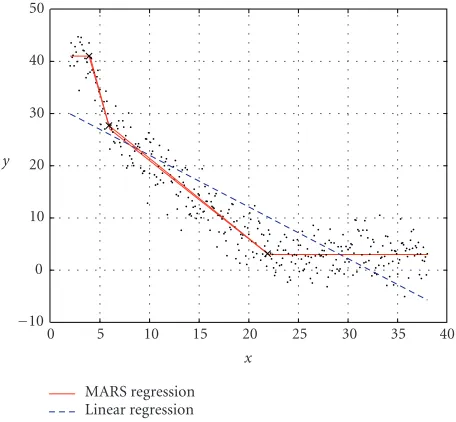
Multivariate adaptive regression spline (MARS) [20] was proposed as an improvement over recursive partitioning al-gorithms such as CART. Unlike CART, MARS produces a continuous regression function f, and the regions of MARS may overlap. In MARS, fis constructed as a sum ofMbasis functions:
f(x)=
M
m=1
amBm(x), (3)
−10 0 10 20 30 40 50
y
0 5 10 15 20 25 30 35 40
x
MARS regression Linear regression
Figure4: A MARS regression function with three knots (marked by×).
where the basis functionBm(x) takes the form of a truncated
spline function. In Figure 4, a single-variable fwith three “knots” is shown, where each knot marks the end of one region of data and the beginning of another. Compared to the linear regression function, the MARS regression function better fits the data.
Clean speech Auditory processing
Degraded speech Auditory processing
Cognitive mapping
Estimated MOS
Figure5: Algorithm architecture.
by an exhaustive search, similar to finding the best split dur-ing CART tree growdur-ing. MARS has been applied to predict customer spending and forecast recession [23], and predict mobile radio channels [24].
3. PROPOSED DESIGN METHOD
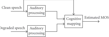
In the proposed method, double-ended measurement algo-rithms are designed based on the architecture depicted in Figure 5. Auditory processing (Figure 6) is first applied to both the clean speech and the degraded speech, to produce a subband decomposition for each signal. The subband de-composed signals and the clean speech signal are input to the cognitive mapping module (Figure 7), where a distortion surface is produced by taking the difference of the two sub-band decompositions. A large pool of candidate feature vari-ables is extracted from the distortion surface. MARS and/or CART is applied to sift out a small set of predictor variables from the pool of candidate variables, while progressively con-structing and optimizing the regression mapping f. This mapping replaces the statistical mining block in Figure 7 upon completion of the design.
The auditory processing modules decompose the input speech signals into power distributions over time frequency and then convert them to auditory excitations on a loudness scale. The cognitive mapping module interprets the diff er-ences (distortions) between the auditory excitations of the clean and the degraded speech signals. In effect, the cogni-tive module “integrates” the distortions over time and fre-quency to arrive at a predicted quality score. We make the simple observation that “distortions are not created equal.” An isolated large distortion event is likely to be cognitively distinct from small distortions that are widely diffused over time frequency, though the small distortions may integrate to a substantial amount. The latter kind of distortion may be less annoying than the former kind. We take an agnostic view of how human cognition weighs the contributions from dif-ferent types of distortions. The approach we take is to create a plethora of “contexts” under which distortion events occur. Distortions with the same context are integrated to a value which we call a “feature.” Straightforward root-mean-square (RMS) integration is used to compute the feature value. Each context gives rise to onecandidatefeature, so that there are as many candidate features as the number of contexts. From the pool of candidate features, data mining techniques are used to find a small subset of features and the best way to
Speech
FFT Power spectrum
Summation over bands
Convert to loudness
Subband decomposed
signal Figure6: The processing steps in an auditory processing module.
combine them to estimate the speech quality. The modules are described next in Sections3.1and3.2. Detailed design considerations and justifications of the modules then follow inSection 3.3, and finally computational complexity is con-sidered inSection 3.4.
3.1. Auditory processing
A block diagram of auditory processing is depicted in Figure 6. Human auditory processing of acoustic signals is commonly modeled by signal decomposition through a bank of filters whose bandwidths increase with filter center fre-quency according to the bark or critical-band scale [8]. A typical realization of this model employs roughly 17 filters or spectral bands to cover the telephone voice channel. In our experiments, we found that 7 bands, each with bandwidth of about 2.4 bark, strike a good balance between prediction performance and sensitivity to irrelevant variations in the in-put data (for further elaboration, seeSection 3.3.1). In our scheme, the speech signal is partitioned into 10-millisecond frames. For each frame, a 128-point power spectrum is cal-culated by applying FFT to a 128-point Hanning-windowed signal segment centering on each frame. The spectral power coefficients are grouped into 7 bands. The coefficients in each band are summed, to produce altogether 7 subband power samples. The samples are converted to subjective loudness scale using Zwicker’s power law [8]:
L(f)=L0
ETQ(f)
s(f)E0 k
1−s(f) +s(f)E(f) ETQ(f)
k
−1
, (4)
where the exponentk=0.23,L0=0.068,E0is the reference excitation power level,ETQ(f) is the excitation threshold at
frequency f,E(f) is the input excitation at frequency f, and s(f) is the threshold ratio.
3.2. Cognitive mapping
Clean speech Clean speech (subband decomposed)
Degraded speech (subband decomposed)
Absolute difference
Distortion VAD & voicing
decision
Severity classification
Contextual distortion integration
Features Statistical data mining
Estimated MOS
Figure7: Cognitive mapping.
the block is replaced by a simple mapping block. The map-ping (the aforementioned f) is computationally simple, as can be seen from the example presented inAppendix B.
3.2.1. Time segmentation
The clean speech signal is processed through a voice activ-ity detector (VAD) and then a voicing detector. Each 10-millisecond speech frame is thereby labeled as either “back-ground,” “active-voiced,” or “active-unvoiced.” We use the VAD algorithm from ITU-T G.729B [25], omitting the com-fort noise generation part of the algorithm. More recent VAD algorithms such as that in the AMR codec [26] may also be used to advantage. The purpose of the segmentation is to sep-arate the different types of speech frames so that they can exert separate influence on the speech quality estimate. The advantage of such segmentation is suggested in [27], where performance was improved using clustering-based segmen-tation.
3.2.2. Severity classification
The total distortion of each frame is classified into different severity levels. The aim is to sift out the significant distor-tion events. Different forms of classifiers can be used. We have experimented with simple thresholding, CART classi-fication [19], and Gaussian mixture density modeling. Based on our simulation results, we have found that a simple clas-sification scheme, thresholding the average frame distortion, suffices to produce most of the benefit. Results presented be-low are based on thresholding to 3 severity levels, which we call low, medium, and high distortion severity. In [28], fixed thresholding of frame energy is shown to provide perfor-mance gain. Gains obtained from classification and segmen-tation are discussed inSection 3.3.2.
3.2.3. Context and aggregation
The speech signal now has a time-frequency representation, with a distortion sample in each time-frequency bin. Each sample is labeled according to its frequency band index, time-segmentation type, and severity level. Contexts are cre-ated by combining label values. For instance, the above seg-mentation and classification creates 7×3×3=63 distinct
values. The distortion samples that have the same composite-label value belong to the same context, which is named af-ter the composite-label value. By associating a context with each distinct composite-label value, we form 63 distinct con-texts. Each context contributes one feature variable to the candidate feature pool to be mined. The value of a feature is obtained via root-mean-square integration of the distor-tion samples in the context, normalized by the number of frames in the speech signal. Thus, each context establishes a specific class of distortion, and contributes to data mining a feature variable which captures the level of the distortion in that class. The feature variables are defined inAppendix A. As an example, the variable U B 2 0 captures the integrated dis-tortion of the context: unvoiced frame, subband 2, and low severity (level 0). We assume that the lengths of the speech signals are no more than several seconds so that recency ef-fects can be ignored. Recency effects can be accounted for by introducing forgetting factors.
3.2.4. Feature pool
Additional contexts are defined in order to create a “rich” pool of candidate features for mining. Besides labeling each frequency subband with its natural subband index, each sub-band is also labeled with the rank order obtained by ranking the 7 distortions in a frame in order of decreasing magnitude. Thus, a candidate feature has either a natural or ordered sub-band index. Rank ordering the subsub-band distortions as well as classifying frame-level distortions based on severity cre-ate contexts that capture distortions independent of specific time-frequency locations, but dependent on the absolute or relative level of distortion severity. This is hypothetically jus-tifiable by the nature of the quality judgment process, and helps the data mining algorithm to pick out cognitively sig-nificant events.
and the highest-frequency-band energy of the clean speech frames, to produce a pool totaling 209 candidate features, as listed inAppendix A. The weighted mean of the 7 subband distortions is calculated using the weights [29]
wi=
1.0 for 0≤i≤4, 0.8 fori=5, 0.4 fori=6.
(5)
The pool of candidate features is redundant for the pur-pose of quality estimation. A brute force approach to find-ing the best subset of features to use would entail examinfind-ing 2209−1 possible subsets, a clearly impossible task. Yet the success of our approach crucially depends on finding a small subset of features that are good for quality estimation. We resort to data mining techniques to perform this task. The effectiveness of the techniques and performance of their de-signs are assessed experimentally inSection 4.
3.3. Feature design and selection
In this section, we present some design justifications.
3.3.1. Number of subbands
We first experimented with using 22 subbands, with each band roughly three-quarter-bark wide. Using CART for re-gression, we found that roughly one out of every three bands was selected. Therefore, we conjectured that we could group the distortions over 22 subbands into a smaller set of 7 sub-band distortions, to achieve a better tradeoffbetween retain-ing relevant spectral information and easy generalization. In a similar rein, reduced spectral resolution was found to im-prove the accuracy of speaker-independent speech recogni-tion [30]. The 2.4-bark bandwidth in our frequency decom-position can also be compared with the 3–3.5 bark critical distance between vowel formant peaks [31].
3.3.2. Design of segmentation and severity classification
In this section, we show the improvements on speech quality estimation due to using segmentation and severity classifica-tion. Estimation performance is assessed using the correla-tion Rand root-mean-square error (RMSE)between the subjective MOSxiand objective MOSyi. Pearson’s formula
gives
R= N
i
xi−x¯
yi−y¯
N
i
xi−x¯
2N
i
yi−y¯
2, (6)
where ¯xis the average ofxi, and ¯yis the average ofyi. RMSE
is calculated using
=
Ni=1
xi−yi
2
N . (7)
The performance results exhibited inTable 1are based on designing a MARS model for a speech database. As we can see, time segmentation alone provides some improvement.
Table1: Performance with different combinations of segmentation and severity classification.
CorrelationR RMSE
No segmentation or classification 0.906 0.306
Segmentation only 0.927 0.273
Severity classification only 0.896 0.339 Segmentation and severity classification 0.977 0.155
An interesting phenomenon is that distortion severity classi-fication alone does not result in any improvement. However, a large improvement is obtained by combining segmentation and classification. We attribute this phenomenon to the dif-ferent significance of a given distortion level across the three types of speech frames: inactive (background noise), voiced, and unvoiced. The signal contents of the three frame types are perceptually very distinct. We expect each type of con-tents to condition the perception of distortion in a certain characteristic fashion. Separating the distortions according to the frame types allows the distortions to be weighed dif-ferently for each type.
For feature definition, we also compared between using (i) the number of distortion samples in a severity class, nor-malized by the number of frames in a speech file, versus (ii) RMS integration of the distortion samples in a severity class. The latter was found to provide better performance.
3.3.3. Feature selection
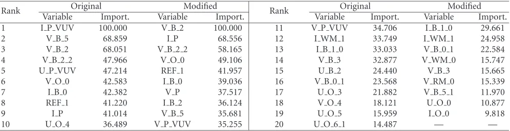
In this section, we acquire a sense of the features selected by MARS by perturbing a MARS designed model. The “Origi-nal” column inTable 2lists the variables of the model being perturbed, in order of decreasing importance. Variable im-portance is determined by the amount of reduction in pre-diction error provided by the variable, relative to the greatest reduction amount achieved amongst all variables. Hence, the variable that results in the largest prediction error reduction has importance 100%, and its amount of error reduction is used as reference. The importance of other variables is cal-culated as the percentage of their prediction error reduction relative to the reference.
Table2: Variable importance list for feature selection investigation. Original: list generated using the full feature pool. Modified: list gener-ated after trimming the feature pool.
Original Modified Original Modified
Rank
Variable Import. Variable Import. Rank Variable Import. Variable Import.
1 I P VUV 100.000 V B 2 100.000 11 V P VUV 34.706 I B 1 0 29.661
2 V B 5 68.859 I P 68.556 12 I WM 1 33.749 I WM 1 24.958
3 V B 2 68.051 V B 2 2 58.165 13 I B 1 0 33.033 V B 0 1 22.584
4 V B 2 2 47.966 V O 0 49.106 14 V B 3 32.877 V WM 0 15.747
5 U P VUV 47.214 REF 1 41.957 15 U B 2 24.440 V B 3 15.665
6 V O 0 42.583 I B 0 39.036 16 V B 0 1 23.568 V RM 0 15.339
7 I B 0 42.382 V P 37.517 17 U O 3 21.882 V B 5 1 11.970
8 REF 1 41.220 I B 2 36.124 18 V O 4 18.121 U O 0 10.877
9 I P 41.014 V B 5 35.681 19 U O 5 15.959 I O 0 9.818
10 U O 4 36.489 V P VUV 35.255 20 U O 6 1 14.487 — —
that both the information captured in a variable as well as the manner of encoding of the information in the variable affect its importance. A rich candidate pool should convey a va-riety of information as well as information encoding. MARS consistently picks out from the available feature variables, the ones with the most relevant information and the best encod-ing. The original model, drawn from a richer pool, is pre-ferred over the modified model. The original model provides root-mean-square prediction error (RMSE) of 0.3902 and 0.3844 on the 90% training database and 10% test database, respectively. (Databases and performance assessment are dis-cussed in the next section.) For the same databases, the modi-fied model achieves RMSE of 0.3968 and 0.4318, respectively.
3.4. Complexity
The computational complexity of the algorithms designed using the proposed approach is mainly attributable to the au-ditory processing modules and to feature extraction process-ing in the cognitive module. While the design of the mappprocess-ing from features to the MOS estimate is somewhat involved, the actual processing needed to realize the mapping once it is de-signed is simple. As the purpose of this paper is to study the application of data mining techniques to design speech qual-ity measurement algorithms, we offer below a rough guide of the algorithm complexity. The actual complexity in specific applications will vary with the details of the features selected. Moreover, as with other measurement algorithms (see, for example, [32]), algorithm complexity may be reducible with-out seriously degrading the estimation accuracy. Such pur-suit of complexity reduction is left to future study.
The complexity of auditory processing in the designed algorithms is no greater than that of the auditory process-ing component in PESQ. A somewhat lower complexity is obtained in our case by using fewer subbands. RMS integra-tion of distorintegra-tion samples to compute the values of the fea-tures employed in the data-mining designed mapping has a roughly similar complexity to theLpintegrations performed
in PESQ. Our use of squared integration throughout, as op-posed to using several different values of p in PESQ, low-ers the integration complexity. Computation of the mapping function (seeAppendix Bfor an example), done only once for the whole speech file, has relatively negligible complexity.
Severity classification also has negligible complexity. The seg-mentation functionalities, VAD and voicing decision, are commonly found in speech coders and other speech pro-cessing applications. We have used the VAD algorithm in ITU-T G.729B [25], omitting its comfort noise generation functionality. We estimate that the segmentation function-alities require no more than 20% of the processing time of the ITU-T G.729 speech codec. The processing time of PESQ is roughly 2.8 times that of G.729. We note that PESQ pro-vides additional functionalities such as variable delay com-pensation. Hence, a speech quality estimator using an algo-rithm designed using the proposed approach while providing a similar suite of functionalities as PESQ would incur a 7% higher complexity than PESQ. As this is a conservative upper bound, we believe complexity implementations lower than PESQ are readily achievable.
4. EXPERIMENT RESULTS
The effectiveness of the data mining approach is demon-strated experimentally with actual designs. We compare the performance of the algorithms designed using our method to the current state-of-the-art algorithm in voice quality esti-mation, PESQ. Below, we first introduce the speech databases used for the experiments. Then we compare the designs ob-tained using different data mining techniques, namely CART, hybrid CART-MARS, and MARS. We finally focus on the method that offers the best performance: MARS design us-ing cross validation. The greatest difference between our de-signed algorithms and PESQ is in the cognitive mapping part; thus, the comparisons below can be regarded as eval-uating different cognitive mappings.
4.1. Speech databases
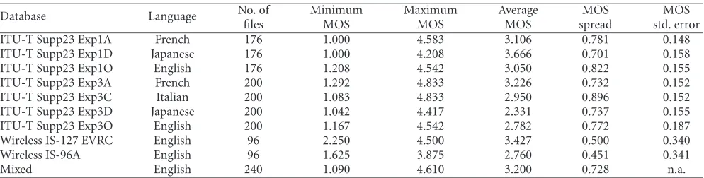
Table3: Properties of the speech databases used for experiments.
No. of Minimum Maximum Average MOS MOS
Database Language
files MOS MOS MOS spread std. error
ITU-T Supp23 Exp1A French 176 1.000 4.583 3.106 0.781 0.148
ITU-T Supp23 Exp1D Japanese 176 1.000 4.208 3.666 0.701 0.158
ITU-T Supp23 Exp1O English 176 1.208 4.542 3.050 0.822 0.155
ITU-T Supp23 Exp3A French 200 1.292 4.833 3.226 0.732 0.152
ITU-T Supp23 Exp3C Italian 200 1.083 4.833 2.950 0.896 0.152
ITU-T Supp23 Exp3D Japanese 200 1.042 4.417 2.331 0.737 0.155
ITU-T Supp23 Exp3O English 200 1.167 4.542 2.782 0.772 0.187
Wireless IS-127 EVRC English 96 2.250 4.500 3.427 0.500 0.340
Wireless IS-96A English 96 1.625 3.875 2.760 0.451 0.341
Mixed English 240 1.090 4.610 3.200 0.728 n.a.
The three Exp1x databases in ITU-T Supp23 contain speech coded using the G.729 codec, singly or in tan-dem with one or two other wireline or wireless standard codecs, under the clean channel condition. Also included are single-encoded speech using these standard codecs. The four Exp3x databases contain single- and multiple-encoded G.729 speech under various channel error conditions (BER 0%– 10%; burst and random frame erasure 0%–5%) and input noise conditions (clean, street, vehicle, and hoth noises at 20 dB SNR).
The wireless IS-96A and IS-127 EVRC (Enhanced Vari-able Rate Codec) databases contain speech coded using the IS-96A and IS-127 codecs, respectively, under various clean and degraded channel conditions (forward FER 3%, re-verse FER 3%), with or without the G.728 codec in tan-dem, and MNRU (modulated noise reference unit) condi-tions of 5–25 dB. The mixed database [18] contains speech coded with a variety of wireline and wireless codecs, under a wide range of degradation conditions: tandeming, chan-nel errors (BER 1%–3%), and clipping (see [18] for more details). All databases include reference conditions such as speech degraded by various levels of MNRU.
The range of the MOSs in each database is determined by its mix of test conditions. The range is characterized in Table 3by the maximum, minimum, average, and “spread”, which is the standard deviation of the MOSs around the aver-age. The imprecision of the subjective MOS is characterized by its standard error (“MOS std. error” inTable 3, which is determined by the number of listeners who participated in the subjective test). The RMSE of the objective scores can be assessed no better than the standard error of the subjective scores used to benchmark the accuracy. Moreover, the mea-surement accuracy of algorithms trained using a database is also limited by the imprecision of its subjective scores. Note that “No. of files” inTable 3refers to the number of speech files that are subjectively scored; the “clean original” speech files are not counted.
The designs presented in this paper are based on the above databases which cover a range of waveform codecs, wireline and wireless LPAS [14] codecs, and a range of codec tandeming and channel error conditions, and input back-ground noise conditions. Additional impairments that can be found in telephone connections but are not currently covered by our databases include echo, variable delay, tones,
distortions due to harmonic or sinusoidal coders and due to music and artificial speech, and so forth the reader can also consult [5] for its list of transmission impairments. The pro-posed design method is highly automated and should scale well with the amount of database material available for de-sign (seeSection 4.6).
4.2. CART results
We first experimented with using CART for mining, moti-vated by the fact that CART results are easier to interpret than MARS results, and CART can be regarded as a special case of MARS. For CART mining, we randomly assigned 90% of the global database to a training data set and the rest to a test data set. The tree-growing phase uses the training set, and the tree-pruning phase uses the test set to select the best-size tree, that is, the one that gives the lowest regression error on the test data. The CART-designed tree has 38 leaf nodes. The per-formance scores areR=0.8861 and=0.3734 on the train-ing set, andR=0.7627 and =0.5098 on the test set. The large difference in RMSE values between training and test-ing indicates that the designed CART tree does not general-ize well. For PESQ, we use the PESQ-LQ mapping suggested in [34] to obtainR =0.8170 and =0.4705 on the global undivided set,R = 0.8198 and =0.4700 on the training set, andR=0.7939 and=0.4744 on the test set. It appears that CART regression trees cannot outperform PESQ.
4.3. Hybrid CART-MARS results
By inspecting the variables mined using CART, we expect them to be perceptually important. The poor performance might be due more to the aforementioned limitations of CART in regression, rather than to the feature selection. Thus, we experimented with using MARS to circumvent the limitations of CART. Below, we present the results from two hybrid CART-MARS schemes.
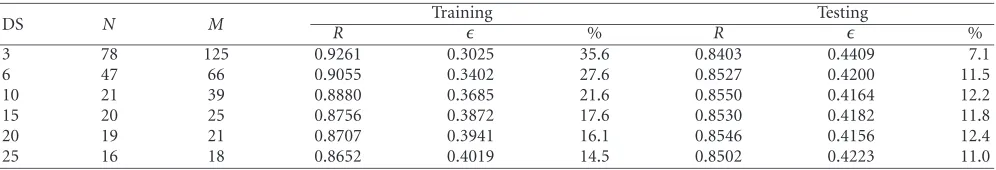
Table4: MARS model selection as a function of DS using 10-fold cross-validation.
Training Testing
DS N M R % R %
3 78 125 0.9261 0.3025 35.6 0.8403 0.4409 7.1
6 47 66 0.9055 0.3402 27.6 0.8527 0.4200 11.5
10 21 39 0.8880 0.3685 21.6 0.8550 0.4164 12.2
15 20 25 0.8756 0.3872 17.6 0.8530 0.4182 11.8
20 19 21 0.8707 0.3941 16.1 0.8546 0.4156 12.4
25 16 18 0.8652 0.4019 14.5 0.8502 0.4223 11.0
The second hybrid CART-MARS method is similar to the method used in [35]. In [35], the feature candidate pool for MARS mining is augmented by the “leaf-node index” ob-tained from a CART tree. We improve on the method by adding the CART regression output variable, instead of the node index variable, to the candidate feature pool. The aug-mented candidate pool is used for MARS model building. In this method, if the CART output were incorporated into the MARS model, feature extraction for the model would also include computation as prescribed by the CART tree. Indeed, an inspection of the variable importance list found that the CART tree output is the most important feature variable selected. The performance obtained, R = 0.9108 and = 0.3326 on the training set, and R = 0.8231 and = 0.4423 on the test set, is also better than PESQ and CART regression. The larger difference between training and testing RMSE in this “augmentation” method, in compari-son with the earlier “prescreening” method, suggests that the “prescreening” method is more robust.
Although both hybrid CART-MARS methods outper-form PESQ and CART, they are inferior to the MARS model of Section 3.3.3 on the test set. In the rest of this paper, we present detailed results based on using MARS alone, as MARS tends to offer the best performance. For the applica-tion in [35], a hybrid CART-MARS scheme provides better performance than CART or MARS alone. Thus, we should not eliminate the possibility of some hybrid schemes outper-forming MARS-only schemes.
4.4. MARS model selection via cross-validation Picking the size of the regression model is a crucial step in the design. The size of the model designed using MARS is a function ofM, the number of basis functions in (3). For lin-ear spline basis functions, two real parameters are associated with each function, the “knot” and the linear combination weight. (Please refer to the example in Appendix B.) Thus, the number of optimized parameters, 2M, is a useful mea-sure of model size. A large model yields low regression error, but the model is highly biased towards the training data and exhibits large variance over unseen data. On the other hand, a small model might omit some important features neces-sary for high measurement accuracy. In Friedman’s original MARS design [20], a penalty term controlled by a “degree of smoothness” (DS) parameter is used in the criterion func-tion to penalize the increased variance due to large model size. Larger DS results in more basis functions taken out during the pruning phase. Friedman’s design method does
not incorporate validation of the model through testing with data not used in model building. We improve on Friedman’s design by using cross-validation to select the model size.
In conventional model design, available data is split into a training set and a test set. The model is built on the for-mer, and validated on the latter. However, when the amount of available data is small, as in our case, we ought to use all the data for model building. Using a small sample to design and validate can be achieved byn-fold cross-validation [36]. The results presented below are based onn=10-fold cross-validation. The global database is randomly divided into 10 data sets with almost equal size. Training and testing is per-formed 10 times. Each time, one of the data sets serves as the test set, and the remaining 9 data sets combined serve as the training set. Each data set serves as a test set only once. For each training-test set combination, a series of MARS mod-els corresponding to various DS values are constructed using the training set. The 10Randvalues obtained for each DS value are averaged to obtain the cross-validationRand val-ues; separate averages are obtained from the training and test sets. Finally, the DS value corresponding to the best cross-validation performance is used to build the desired MARS model using the entire global database.
Table 4 shows the cross-validation performance results for a series of MARS models obtained using different values of DS. Both training and test results are shown, withN de-noting the average number of distinct feature variables used in the cross-validation models,Mthe average number of ba-sis functions, and % the average percentage reduction in compared to PESQ. FromTable 4, we pick the best DS value for designing our final model. We see that for DS =20, the RMSE reduction is the largest, and the discrepancy between the training and test performance is the smallest. Thus, the final model is built using the global database, with DS=20.
Table5: Variable importance ranking for the global model.
Rank Variable Importance Rank Variable Importance Rank Variable Importance
1 V RM 100.00 8 I B 0 39.782 15 U O 4 24.530
2 I P 76.280 9 I B 1 0 37.531 16 U O 5 22.092
3 V B 2 2 56.375 10 V O 0 37.143 17 V P 1 21.172
4 REF 1 50.151 11 V B 2 36.379 18 U B 4 19.639
5 V P 44.425 12 V O 5 33.179 19 V B 0 1 17.459
6 V O 0 2 41.897 13 I WM 1 31.807 20 U O 6 1 17.048
7 V P VUV 40.472 14 V P 2 25.562 21 I B 5 15.592
Table6: MARS model performance on the 10 speech databases: variation over samples.
CorrelationR RMSE Percentage
Database Language
Proposed Method PESQ Proposed Method PESQ reduction in(%)
ITU-T Supp23 Exp1A French 0.8753 0.8498 0.3909 0.4507 13.3
ITU-T Supp23 Exp1D Japanese 0.9141 0.8725 0.3988 0.5893 32.3
ITU-T Supp23 Exp1O English 0.8998 0.9164 0.3581 0.3616 1.0
ITU-T Supp23 Exp3A French 0.8480 0.8199 0.4327 0.5482 21.1
ITU-T Supp23 Exp3C Italian 0.9099 0.8935 0.4048 0.4499 10.0
ITU-T Supp23 Exp3D Japanese 0.8728 0.8965 0.4127 0.5366 23.1
ITU-T Supp23 Exp3O English 0.8757 0.8857 0.3749 0.4222 11.2
Wireless EVRC English 0.6364 0.5522 0.3952 0.4359 9.3
Wireless IS-96A English 0.5786 0.4562 0.3845 0.4282 10.2
Mixed English 0.8771 0.8732 0.3496 0.4083 14.4
Average — — — — — 14.6
the logarithmic spectral distortion that speech spectral quan-tizers are generally designed to minimize [14]. V B 2 2 is the RMS distortion in subband 2 of the voiced frames that have the highest severity of frame distortion. Subband 2 covers the frequency region where the long-term power spectrum of speech peaks. V O 0 2 is the RMS distortion in the highest-distortion subband of the voiced frames that have the highest severity of frame distortion; in effect, V O 0 2 measures the intensity of peak distortions. The selection of V B 2 2 and V O 0 2 suggests that speech quality perception is strongly dependent on prominent spectral regions and distortion events. The variables I P, V P, and V P VUV, which measure the relative amount of specific frame types, and REF 1, which measures the level of high-frequency loudness in the refer-ence signal, serve to adjust the regression mapping. For in-stance, inAppendix B, we see that the predicted quality value is raised when the fraction of inactive frames is above 0.27, and is decreased when the fraction drops below 0.27.
4.5. Database results
We apply the global model to the individual databases listed inSection 4.1. We report performance results in two formats: variation over samples (VOS) inTable 6, and variation over conditions (VOC) in Table 7. In VOS, the correlation and RMSE between the objective and subjective MOS of each sample is reported. A “sample” refers to a pair of speech files used for quality calculation: the speech file that was played to the listener panel, and the “clean” original version of the speech that was played. For VOC, the subjective MOSs for the speech files within the same test condition are first averaged together.
The objective MOSs are also likewise grouped and aver-aged. Then,Randare calculated between the per-condition averaged subjective and objective MOSs, over all conditions in the database. The VOS results better reflect performance in voice quality monitoring applications [3]. The VOC re-sults are more appropriate for codec or transmission equip-ment evaluation. To the best of our knowledge, all the per-formance results that have been reported in the literature for PESQ by its inventors use the VOC format. The results for PESQ are based on using the PESQ-LQ 3rd-order regression polynomial specified in [34]. The results in Tables 6and7 show that the global model provides an average reduction in RMSEof 14.6% and 21.4%, for VOS and VOC averaging, respectively.
We adopt the simple model proposed in [7] to help us in-terpret the relationship between theRandvalues in Tables 6 and7; the model is modified with the addition of a bias term. Accordingly,Randsatisfy the following relationship:
2=
σ21−R2+σMOS2 +b2, (8)
whereσ2andσ2
MOS are the “MOS spread” and “MOS std. Error” inTable 3, respectively, andbis systematic bias. The equation states that 2 is the sum of unexplained variance in the estimation model, MOS estimation error due to lim-ited number of listeners, and bias error between subjective and objective MOSs. In comparing estimation algorithms us-ing the same databases,σ2
Table7: MARS model performance on the 10 speech databases: variation over conditions.
CorrelationR RMSE Percentage
Database Language
Proposed Method PESQ Proposed Method PESQ reduction in(%)
ITU-T Supp23 Exp1A French 0.9381 0.9343 0.2769 0.3609 23.3
ITU-T Supp23 Exp1D Japanese 0.9391 0.9539 0.2595 0.5136 49.5
ITU-T Supp23 Exp1O English 0.9644 0.9566 0.2441 0.2705 9.8
ITU-T Supp23 Exp3A French 0.9400 0.8776 0.3109 0.4743 34.5
ITU-T Supp23 Exp3C Italian 0.9508 0.9455 0.3243 0.3441 5.8
ITU-T Supp23 Exp3D Japanese 0.9455 0.9452 0.2888 0.4785 39.6
ITU-T Supp23 Exp3O English 0.9459 0.9254 0.2551 0.3522 27.6
Wireless EVRC English 0.8224 0.8116 0.2139 0.2176 1.3
Wireless IS-96A English 0.6323 0.6203 0.2371 0.2250 −5.4
Mixed English 0.9364 0.9188 0.2438 0.3366 27.6
Average — — — — — 21.4
0
1A 1D 1O 3A 3C 3D 3O
0.2 0.4 0.6 0.8 1
Database 7 databases
10 databases
Cor
re
la
ti
o
n
R
(a)
0
1A 1D 1O 3A 3C 3D 3O
0.05 0.1 0.15 0.2 0.25 0.3 0.35 0.4
Database 7 databases
10 databases
RMSE
(b)
Figure8: Comparison of MARS model performance between training on the 7 ITU-T databases and on all 10 speech databases. (a) Corre-lation and (b) RMSE results are shown for variation over conditions.
and Exp3D, even thoughRis quite high for databases Exp1D and Exp3D. According to (8), the largevalues can be due to bias errors, which we attribute to biases between individ-ual databases and the global database. The MARS model is able to adjust for individual databases, thus reducing the bias component.
4.6. Scalability
It is highly desirable to be able to design models that can scale with the amount of data available for learning. Also, new forms of speech degradations arise as a result of new transmission environments, new speech codecs, and so forth. The data mining approach enables designing best-size mod-els for a given amount of learning data, and adapting to new learning data. To demonstrate the scalability of the proposed method, we created a smaller global database comprising
5. CONCLUSION
We have proposed an approach to design objective speech quality measurement algorithms using statistical data mining methods. We have examined various methods of using CART and MARS to design novel objective speech quality measure-ment algorithms. The methods select feature variables from a large pool to form speech quality estimation models. We have obtained designs that outperform the state-of-the-art stan-dard PESQ algorithm in our databases. The variables form-ing the models are found to be perceptually significant, and the methods offer some insights into the relative importance of the variables. The designed algorithms are computation-ally simple, making them suitable for real-time implemen-tation. The best performing algorithm was designed using MARS.
We also showed that the proposed design method can scale with the amount of learning data. The experience learned from building training-based systems such as speech recognizers suggests using that the performance of the algo-rithms designed using our approach can be substantially im-proved with large-scale training, offline or online. The algo-rithms also show promise for further optimization and com-plexity reduction. The design approach can be extended to other media modalities such as video.
APPENDICES
A. FEATURE VARIABLE DEFINITIONS
The feature variables are defined below. The first letter, de-noted by T in a variable name, gives the frame type: T = I for Inactive, T = V for Voiced, and T = U for Unvoiced. The subband index is denoted byb, withb ∈ {0,. . ., 6} in-dexing from the lowest to the highest frequency band if the index is natural, or from the highest to the lowest distortion if the index is rank-ordered. The frame distortion severity class is denoted byd, withd ∈ {0, 1, 2}indexing from low-est to highlow-est severity. With the above notations, the feature variables are as follows.
(i) T Pd: fraction of T frames in severity classdframes. (ii) T P: fraction of T frames in the speech file.
(iii) T P VUV: ratio of the number of T frames to the total number of active (V and U) speech frames.
(iv) T Bb: distortion for subbandbof T frames, without distortion severity classification, for example, I B 1 represents subband 1 distortion for inactive frames. (v) T Bb d: distortion for severity classdof subbandbof
T frames, for example, V B 3 2 represents distortion for subband 3, severity class 2, of voiced frames. (vi) T Ob: distortion for ordered subbandbof T frames,
without severity classification, for example, U O 3 represents ordered-subband 3 distortion for unvoiced frames, without distortion severity classification. (vii) T Ob d: distortion for distortion classd of ordered
subbandbof T frames, for example, U O 6 1 repre-sents distortion for severity class 1 of ordered-subband 6 of unvoiced frames.
(viii) T WMd: weighted mean distortion for severity class dof T frames.
(ix) T WM: weighted mean distortion for T frames. (x) T RMd: root-mean distortion for severity classdof T
frames.
(xi) T RM: root-mean distortion for T frames.
(xii) REF 0: the loudness of the lower 3.5 subbands of the reference signal.
(xiii) REF 1: the loudness of the upper 3.5 subbands of the reference signal.
B. GLOBAL MARS MODEL
The basis functions BFn, wherenis an integer, and the re-gression equation of the global model are listed below:
BF3=max(0, I P−0.270); BF4=max(0, 0.270−I P); BF6=max(0, 33.581−REF 1); BF8=max(0, 0.725−V B 2); BF10=max(0, 0.131−I B 0); BF12=max(0, 1.731−V B 2 2); BF13=max(0, V P 2−0.710); BF17=max(0, I WM 1−0.177); BF20=max(0, 0.758−V P VUV); BF23=max(0, V P−0.422); BF24=max(0, 0.422−V P); BF25=max(0, V O 0−2.284); BF28=max(0, 0.031−U O 6 1); BF30=max(0, 0.134−I B 5); BF41=max(0, V RM−0.786); BF42=max(0, 0.786−V RM); BF44=max(0, 0.070−I B 1 0); BF50=max(0, 0.390−U O 4); BF52=max(0, 1.657−U B 4); BF62=max(0, 0.132−U O 5); BF68=max(0, 0.331−V P 1);
BF75=max(0, V B 0 1−0.337061E-08); BF154=max(0, V O 0 2−2.036); BF169=max(0, V O 5−0.548); Objective MOS
=2.534 + 6.738∗BF3−1.833∗BF4
ACKNOWLEDGMENTS
We thank Nortel Networks for their financial support. We also thank the reviewers for helping to substantially improve the presentation in this paper.
REFERENCES
[1] D. G. Jamieson, V. Parsa, M. Price, and J. Till, “Interaction of speech coders and atypical speech, II: effects on speech qual-ity,”Journal of Speech Language & Hearing Research, vol. 45, pp. 689–699, 2002.
[2] N. Kitawaki and H. Nagabuchi, “Quality assessment of speech coding and speech synthesis systems,”IEEE Commun. Mag., vol. 26, no. 10, pp. 36–44, 1988.
[3] A. E. Conway, “A passive method for monitoring voice-over-IP call quality with ITU-T objective speech quality measure-ment methods,” in Proc. IEEE International Conference on Communications (ICC ’02), vol. 4, pp. 2583–2586, New York, NY, USA, April–May 2002.
[4] ITU-T Rec. P.800, “Methods for subjective determination of transmission quality,” International Telecommunication Union, Geneva, Switzerland, August 1996.
[5] ITU-T Rec. P.862, “Perceptual evaluation of speech quality (PESQ): an objective method for end-to-end speech quality assessment of narrow-band telephone networks and speech codecs,” International Telecommunication Union, Geneva, Switzerland, February 2001.
[6] ITU-T Rec. P.563, “Single ended method for objective speech quality assessment in narrow-band telephony applications,” International Telecommunication Union, Geneva, Switzer-land, May 2004.
[7] R. F. Kubichek, D. Atkinson, and A. Webster, “Advances in objective voice quality assessment,” inProc. IEEE Global Telecommunications Conference (GLOBECOM ’91), vol. 3, pp. 1765–1770, Phoenix, Ariz, USA, December 1991.
[8] E. Zwicker and H. Fastl, Psychoacoustics: Facts and Models, Springer-Verlag, New York, NY, USA, 2nd edition, 1990. [9] S. Voran, “Objective estimation of perceived speech quality. I.
Development of the measuring normalizing block technique,” IEEE Trans. Speech Audio Processing, vol. 7, no. 4, pp. 371–382, 1999.
[10] S. Voran, “Objective estimation of perceived speech quality. II. Evaluation of the measuring normalizing block technique,” IEEE Trans. Speech Audio Processing, vol. 7, no. 4, pp. 383–390, 1999.
[11] S. Wang, A. Sekey, and A. Gersho, “An objective measure for predicting subjective quality of speech coders,”IEEE J. Select. Areas Commun., vol. 10, no. 5, pp. 819–829, 1992.
[12] N. S. Jayant and P. Noll,Digital Coding of Waveforms: Princi-ples and Applications to Speech and Video, Prentice-Hall, En-glewood Cliffs, NJ, USA, 1984.
[13] J. E. Schroeder and R. F. Kubichek, “L1and L2normed cepstral
distance controlled distortion performance,” inProc. IEEE Pa-cific Rim Conference on Communications, Computers and Sig-nal Processing (PACRIM ’91), vol. 1, pp. 41–44, Victoria, BC, Canada, May 1991.
[14] W. B. Kleijn and K. K. Paliwal, Eds.,Speech Coding and Syn-thesis, Elsevier Science, Amsterdam, The Netherlands, 1995. [15] S. R. Quackenbush, T. P. Barnwell III, and M. A. Clements,
Objective Measures of Speech Quality, Prentice-Hall, Engle-wood Cliffs, NJ, USA, 1988.
[16] A. W. Rix, J. G. Beerends, M. P. Hollier, and A. P. Hek-stra, “Perceptual evaluation of speech quality (PESQ)—a new method for speech quality assessment of telephone networks and codecs,” inProc. IEEE Int. Conf. Acoustics, Speech, Signal
Processing (ICASSP ’01), vol. 2, pp. 749–752, Salt Lake City, Utah, USA, May 2001.
[17] M. P. Hollier, M. O. Hawksford, and D. R. Guard, “Error ac-tivity and error entropy as a measure of psychoacoustic sig-nificance in the perceptual domain,”IEE Proceedings of Vision, Image and Signal Processing, vol. 141, no. 3, pp. 203–208, 1994. [18] L. Thorpe and W. Yang, “Performance of current perceptual objective speech quality measures,” inProc. IEEE Workshop on Speech Coding Proceedings, pp. 144–146, Porvoo, Finland, June 1999.
[19] L. Breiman, J. H. Friedman, R. A. Olshen, and C. J. Stone, Classification and Regression Trees, CRC Press, Boca Raton, Fla, USA, 1984.
[20] J. H. Friedman, “Multivariate adaptive regression splines,” The Annals of Statistics, vol. 19, no. 1, pp. 1–141, 1991. [21] N. Suzuki, S. Kirihara, A. Ootaki, M. Kitajima, and S.
Naka-mura, “Statistical process analysis of medical incidents,”Asian Journal on Quality, vol. 2, no. 2, pp. 127–135, 2001.
[22] K. O. Perlmutter, S. M. Perlmutter, R. M. Gray, R. A. Olshen, and K. L. Oehler, “Bayes risk vector quantization with pos-terior estimation for image compression and classification,” IEEE Trans. Image Processing, vol. 5, no. 2, pp. 347–360, 1996. [23] P. Sephton, “Forecasting recession: can we do better on MARS?”Federal Reserve Bank of St. Louis Review, vol. 83, no. 2, pp. 39–49, 2001.
[24] T. Ekman and G. Kubin, “Nonlinear prediction of mobile radio channels: measurements and MARS model designs,” inProc. IEEE Int. Conf. Acoustics, Speech, Signal Processing (ICASSP ’99), vol. 5, pp. 2667–2670, Phoenix, Ariz, USA, March 1999.
[25] ITU-T Rec. G.729 - Annex B, “A silence compression scheme for G.729 optimized for terminals conforming to recom-mendation V.70,” International Telecommunication Union, Geneva, Switzerland, November 1996.
[26] ETSI EN 301 708 V7.1.1, “Digital Cellular Telecommunica-tions System (Phase 2+); Voice Activity Detector (VAD) for Adaptive Multi-Rate (AMR) Speech Traffic Channels,” Euro. Telecom. Stds. Inst., December 1999.
[27] R. F. Kubichek, E. A. Quincy, and K. L. Kiser, “Speech quality assessment using expert pattern recognition techniques,” in Proc. IEEE Pacific Rim Conference on Communications, Com-puters and Signal Processing (PACRIM ’91), pp. 208–211, Vic-toria, BC, Canada, June 1989.
[28] S. Voran, “Advances in objective estimation of received speech quality,” inProc. IEEE Workshop on Speech Coding for Telecom-munications, Porvoo, Finland, June 1999.
[29] K. K. Paliwal and B. S. Atal, “Efficient vector quantization of LPC parameters at 24 bits/frame,”IEEE Trans. Speech, and Au-dio Processing, vol. 1, no. 1, pp. 3–14, 1993.
[30] H. Hermansky, “Perceptual linear predictive (PLP) analysis of speech,”Journal of the Acoustical Society of America, vol. 87, no. 4, pp. 1738–1752, 1990.
[31] L. Chistovich and V. V. Lublinskaya, “The ‘center of gravity’ effect in vowel spectra and critical distance between the for-mants: psychoacoustical study of the perception of vowel-like stimuli,”Hearing Research, vol. 1, no. 3, pp. 185–195, 1979. [32] S. Voran, “A simplified version of the ITU algorithm for
objec-tive measurement of speech codec quality,” inProc. IEEE Int. Conf. Acoustics, Speech, Signal Processing (ICASSP ’98), vol. 1, pp. 537–540, Seattle, Wash, USA, May 1998.
[33] ITU-T Rec. P. Supplement 23, “ITU-T coded-speech database,” International Telecommunication Union, Geneva, Switzerland, February 1998.
[35] A. Abraham, “Analysis of hybrid soft and hard computing techniques for forex monitoring systems,” inProc. IEEE Inter-national Conference on Fuzzy Systems (FUZZ-IEEE ’02), vol. 2, pp. 1616–1622, Honolulu, Hawaii, USA, May 2002.
[36] M. Stone, “Cross-validation choice and assessment of statisti-cal predictions,”Journal of the Royal Statistical Society: Series B, vol. 36, pp. 111–147, 1974.
Wei Zhareceived his B.S. and M.S. degrees from Shanghai Jiao Tong University, Shang-hai, China, both in electronics engineering. He worked in the Department of Electron-ics Engineering, Shanghai Jiao Tong Univer-sity, Shanghai, China. He received his Ph.D. degree in electrical and computer engineer-ing from Queen’s University, Kengineer-ingston, On-tario, Canada, in 2002. From 2002 to 2003, he worked on speech quality measurement
at Queen’s University. From 2003 till the end of 2004, he was with the Coordinated Science Laboratory, University of Illinois at Urbana-Champaign, holding an NSERC Fellowship. Since January 2005, he has been with Schlumberger Houston Tech Center.
Wai-Yip Chan (usually known as Geof-frey Chan) received his B.Eng. and M.Eng. degrees from Carleton University, Ottawa, Canada, and his Ph.D. degree from the Uni-versity of California at Santa Barbara, all in electrical engineering. He is currently an Associate Professor of electrical and com-puter engineering at Queen’s University, Kingston, Canada. Previously, he was on the faculty of Illinois Institute of