More on sliding right
Joachim Breitner
DFINITY Foundation, [email protected]
Abstract
This text can be thought of an “external appendix” to the paperSliding right into disaster: Left-to-right sliding windows leakby Daniel J. Bernstein, Joachim Breitner, Daniel Genkin, Leon Groot Bruinderink, Nadia Heninger, Tanja Lange, Christine van Vredendaal and Yuval Yarom [1, 2], and goes into the details of
• an alternative way to find the knowable bits of the secret exponent, which is complete and can (in rare corner cases) find more bits than the rewrite rules in Section 3.1 of [1], • an algorithm to calculate the collision entropyHthat is used in Theorem 3 of [1], and • a proof of Theorem 3.
All errors, typos and irrelevancies in the present paper are purely Joachim Breitner’s fault, and not of any of the other authors of [1, 2].
The Haskell implementation of algorithm can be found at https://github.com/nomeata/slidingright.
1 Knowing all knowable bits
Section 3.1 of [1] describes how to learn some bit of the secret exponent, given the sequence of square and multiply operations performed by Algorithm 2, using four simple rewrite rules. It turns out that these rules are not able to recoverallknown bits. Consider, for example, the bit string
00010010001000100010001010000010001,
producing the sequence
ssssmsssmssssmssssmssssmssssmssmssssssmssssm
which is first converted to
xxxxxxxxxxxxxxxxxxxxxxxxxxxxxxxxxxx
xxx1xx10xx1
a
xx
↑x1bxxx1c
xxx1
d
x1
e
00xxx1xxx1
But every bit sequence leading to the above sequence of squares and multiplies must have a1in the position marked with an arrow!
To see why the most significant bit of the multiplier for multiplicationbmust be there, consider the alternatives. It cannot be one bit earlier, as then it would be included in the window fora. It also cannot be later, i.e. a multiplication with 3 or 1, as then the same would hold forc, and henced, which is not possible, as otherwise the multiplication atdwould include the1ate.
These missed opportunities are rare and do not significantly affect the efficiency of the pruning, but in the interest of completeness, we provide an algorithm to recover the bits which finds all knowable bits.
1.1 Possible window widths
We can find out all knowable bits if we keep track of the possible widths of the multiplier of each observed multiplication. Consider a multiplication at positioni=5, i.e.xxxx1xxxxx. Forw=4, this corresponds to one of four cases:
Case 1: x1xx1xxxxx, multiplier width: 4 Case 2: xx1x10xxxx, multiplier width: 3 Case 3: xxx1100xxx, multiplier width: 2 Case 4: xxxx1000xx, multiplier width: 1
The key idea is now thatmultipliers do not overlap. More precisely, if the multiplier of the multiplication at positionihas widthmi and the multiplier of the multiplication at position j
has widthmj(withi>j), then
i+mi−w≥j+mj.
From this, we can derive a simple linear algorithm that calculates the possible multiplier widths for each multiplication. We define
• m−i to be the smallest possible width of the multiplication at positioni, and • m+
i to be the largest possible width of the multiplication at positioni.
LetM={k0,k1, . . . ,kn}be the positions of the multiplications, withk0> · · · >kM. Then
m−k
i= (
1, ifi=n
max(1,ki+1+m−
ki+1+w−ki), otherwise, and
m+k
i= (
w, ifi=0
min(w,ki−1+m+k
i−1−w−ki), otherwise.
Givenm−andm+, we can calculate all the knowable bits of the input sequence. Let us represent this bybi∈{0,1,x}, defined as follows:
bi=
1, ifi∈M
1, else if j+m−j−1=i=j+m+j−1 for some j∈M
x, else if j+m−j−1≤i≤j+m+j−1 for some j∈M
0 otherwise.
The first case corresponds to Rule 0 in Section 3.1 of [1] (last bit), the second to Rule 2 (first bit) and the last case to Rules 1 and 3 (trailing and leading zeroes).
Theorem 1 This algorithm is correct and complete.
This means not only that the input sequence have bitiset according tobi, but also that ifbi=x,
then there are two input sequence that produce the given sequence of squares and multiplies and differ at biti. In other words: All knowable bits are known.
PROOF(SKETCH) Correctness follows by construction of the algorithm. Completeness, because for every unknown bit (x) we can construct two sequences, one with a1and one with a0in that spot, that map to the same square-and-multiply sequence.
Example For the input above, withw=4, we learn
Input: xxxxxxxxxxxxxxxxxxxxxxxxxxxxxxxxxxx
m−: 4 3 3 3 3 3 1 1 1
m+: 4 3 3 3 3 3 1 3 3
bi: 1xx11x101x101x101x101x101000xx10xx1.
1.2 Self-information
Calculating m+ and m− not only allows us to read off all knowable bits, it also allows us to calculate the number of input sequences that produce the given sequence of squares and multiplies.
We define the function f(i,z) to be the number of colliding sequences for the output including the window at positionki, under the additional constraint that the earliest1occurs at positionz. This
function is recursively defined (and admits to a straight-forward efficient dynamic programming implementation). The base case is f(i,z)=1 fori>n, otherwise we have
f(i,z)=
m+
ki X
m=m−
ki
[ki+m−1≤z]·2max(0,m−2)·f(i+1,ki+m−1−w)
where
• the sum iterates over all possible multiplier widths at this position,
• the power of two takes into account the unknown bits in this window,
• and the recursive call goes to the next window, updating the constraint on the next allowed1.
The total number of colliding sequences is then f(0,l), wherelis the length of the input, and the self-information of the sequence isIs= −logps= −logf(0,2ll).
Example For the example above, this yields 1408 possible input sequences, a self-information of 24.5, and hence 0.70 bits of self-information per bit of input. Note that 1408 is not simply two to the number ofx: not all assignments to yield valid input sequences.
2 Calculating the collision entropy of a leak
From Theorem 3 of [1] we learn that the expected search tree size depends on thecollision entropy rate Hof the square-and-multiply sequence. While we are not able to give a closed formula ofH
in the window widthw, we can calculate it for a givenw. The individual steps are
1. Create a Mealy automaton that converts the bits of the secret exponent into a sequence of squares and multiplies.
2. Turn this automaton into an equivalent Hidden Markov Chain, by delaying the output by
wbits.
3. Calculate the collision entropy of the Markov chain by finding the stationary distribution of the colliding process.
Just as Theorem 3 applies to partial information beyond sliding windows, we believe that this approach will be useful to analyze other information leaks.
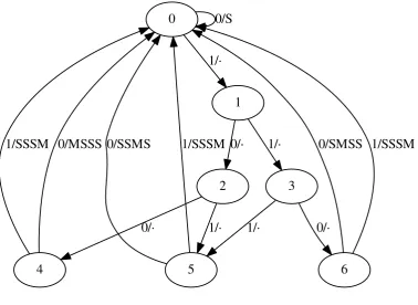
2.1 A Mealy automaton
We can model the sequence of squares and multiplies performed by Algorithm 2 in [1] as a mealy automaton with input alphabetΣ={0,1}and output alphabetΓ∗={S, M}∗(where M represents a combined square-and-multiply sequence). Because the algorithm may scan up to the nextw
bits, we can use the 2w−1 statesS={0, . . . , 2w−1−1} to build the automaton in a straight-forward manner, where the state number directly encodes the bits scanned:
State Input Output Next state
0 0 S 0
0 1 1
0<x<2w−2 0 2·x
0<x<2w−2
0
0/S
1
1/·
2
0/·
3
1/·
4
0/·
5
1/·
1/·
6
0/·
0/MSSS
1/SSSM
0/SSMS
1/SSSM
0/SMSS 1/SSSM
Figure 1: Mealy automaton,w=4
Oncewbits are scanned into x, the sequence of squares and multiplies corresponding toxis printed, defined by
SM(x) :=Sw−i−1MSi,
whereiis the position of the last1inx, and the algorithm continues again in state 0.
Some states are actually equivalent, such as 5 and 7 forw=4, because the algorithm does not distinguish between the bit sequence101and111, and a standard automaton reduction algorithm can coalesce these nodes. Forw=4, this the resulting automaton is shown in Figure 1.
2.2 Mealy automaton to Markov chain
SSSS0
SSS1
SS2
SS3 S4
S5 S6
SSSM0
MSSS0 SSMS0
SSM1
SMSS0
SMS1 MSS1
SM2 SM3
MS2 MS3
M4
M5 M6
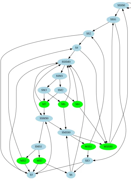
In all generality: Given a Mealy automaton with state spaceS, input alphabetΣ, output alphabet Γ∗, output functionρ:S×Σ→Γ∗and transition functionδ:S×Σ→S, we can construct a Markov chain with state spaceS0:=S×Γ∗which has transitions
(γ1γ2,s)−→(γ2ρ(s,i),δ(s,i))
forγ1∈Γ,γ2∈Γ∗,s∈Sandi∈Σwith probability |Σ|1 . This is a hidden state Markov chain, where
only the first symbolγ1of a state (γ1γ2,s) is visible. We restrict the Markov chain to the states reachable from a sensibly chosen start state; in our case that is (Mw, 0).
This process turns the mealy automaton from Figure 1 into the Markov chain shown in Figure 2. The colors indicate the visible state of each node: green for M, blue for S.
At this point it becomes irrelevant which input bit (0or1) causes a transition, as we are interested in the distribution of the output.
2.3 Collision entropy of a Markov chain
The final step is to calculate the collision entropy of a hidden Markov chain. To that end, we construct a Markov chain that simulates the evolution of two independent instances of the given Markov chain, find the stationary distribution of still-colliding states and calculate the probability of the two Markov chains producing different output in the next step. More theoretical details and generalizations of this novel approach can be found in [3].
We start with a Markov chain with state spaceS, transition probability p:S→S→Rand visible stateρ: :S→Γ.
The product Markov chain has state spaceS×Sand transition probability
p¡
(s1,s2), (s01,s02)
¢
=p(s1,s01)·p(s2,s02).
We find a probability distributionP:C→Ron the colliding states
C:={(s1,s2)∈S×S|ρ(s1)=ρ(s2)}
that is stationary in the sense that if the product Markov chain starts in this distribution, takes a step and ends up in a state inCagain, then it is again in this distribution. In other words, it satisfies the equation
P(s)= X
s0∈C
P(s0)·p(s0,s)
X
s0,s∈C
P(s0)·p(s0,s).
for alls∈C. The denominator re-normalizes the distribution, as the next state may not be in
C. We can find this distribution as the eigenvector with the largest eigenvalue of the transition matrix of the product Markov chain with all transitions outside ofCset to zero. (In contrast to the usual stationary distribution of a Markov chain, the eigenvalue will be smaller than 1.)
The collision probability rate is now simply the probability of the product Markov chain remaining inC, and hence the collision entropy rate is:
H= −log X
s0,s∈C
1 2 3 4 5 6 7 0
0.2 0.4 0.6 0.8 1
w
H
Left-to-right Right-to-left
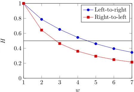
Figure 3: Collision entropy rate
2.4 Results
We have applied this process to both left-to-right and right-to-left sliding window leaks for various window widths, and obtain the following results, which are also plotted in Figure 3. We can see that forw=4, compared to right-to-left, left-to-right hoists the collision entropy rate over the threshold of 0.5, and forw=5 moves it very close.
w 1 2 3 4 5 6 7
left-to-right 1.000 0.786 0.652 0.545 0.460 0.395 0.345 right-to-left 1.000 0.643 0.463 0.360 0.294 0.249 0.215
2.5 Why not Shannon entropy?
In Theorem 3 and this section, we are are concerned with the collision entropy, also known as as Rényi entropy [5], rather than the more common Shannon entropy. Why is this the case? Let us recall the definition of the Shannon entropyH1 and the collision entropy H2 for a random
variableX withpx=P(X=x):
H1:= −
X
x
px·logpx H2:= −log
X
x
p2x
We always haveH2≤H1, and equality for an uniformly distributedX.
Note thatP
xp2x=P(X1=X2), the probability of two independent random variables with the
same distribution asX to coincide, hence the namecollision entropy. And it is exactly when there is a collision between the partial information from the actual secret key and from the guessed suffix when the pruning algorithm will carry on.
3 Proof of Theorem 3
We can prove Theorem 3 of [1] in a more general setting than just left-to-right leakage: We assume an oracle that, given a hypothesized suffixp0ofd
pof lengthntells us whether this is
indeed a possible suffix. This framework allows us to model various forms of partial information aboutdp, including randomly known bits and square and multiply sequences.
In notation: An(dp,d0p) holds if the oracle does not refute thenleast significant bits ofd0pas a
possible suffix ofdp.
Assumption Our proof relies on these assumptions:
1. If we guessedd0pandd0qwrong, and the least significant wrongly guessed bit is at position
i, then we assume that the probability that the RSA equation
RSAn(dp,dq) :=(edp−1+kp)(edq−1+kq)=kpkqN mod 2n
holds to be 2−(n−i).
2. In the above situation, we assume that the probability of the oracles fordpanddq to accept
the guesses after the first wrongly guessed bit are independent.
3. The probability of the oracle accepting ann-bit suffix where the last ibits are correct is less than the probability of the oracle accepting a random (n−i)-bit suffix:
P(An(dp,d0p)|lastibits ofd0pare correct)≤P(An−i(dp,d0p))
4. The probability of the oracle accepting a next bit is constant. In other words,
P(An(dp,dq))=2−nH
for someH∈[0, 1]. The constantHcan be understood as the collision entropy rate of the oracle.
It suffices if these assumptions hold for almost alln; if they do not hold for smallnthen the inequality in Theorem 3 holds up to a constant factor.
Proof We use some additional notation: Letkbe the key size, i.e. the lengths of both p,q∈{0, 1}k. We use (x,y)6=n(x0,y0) to denote that then least significant bits ofxandx0 and of yand y0 are equal, and that then’th bit of eitherxandx0or yand y0 differ.
In general, the size of a search tree with pruning is
S(dp,dq) :=
k−1
X
n=0
X
d0
p,d0q∈{0,1}n
[OKn(dp,dq,d0p,d0q)]
where the predicate OK is true if the least significantnbits ofd0pandd0qare potentially correct suffixes of the actual valuesdpanddq. In our case,
This notion of size counts all nodes of the tree that are not pruned, i.e. excludes the leaves where a contradiction is observed.
We can further split this sum up according to whether we guessed all bits correctly (in which case [OKn(dp,dq,d0p,d0q)]=1) or if not, when was the first bit that we guessed wrongly:
S(dp,dq)= k−1
X
n=0
1+
n
X
i=0
X
d0
p,d0q∈{0,1}n
[(d0p,d0q)=6i (dp,dq)∧OKn(dp,dq,d0p,d0q)]
.
Reordering the sum to iterate over the position of the wrongly guessed bit first, we get
S(dp,dq)=k+ k−1
X
i=0
k−1
X
n=i
X
d0
p,d0q∈{0,1}n
[(d0p,d0q)=6i (dp,dq)∧OKn(dp,dq,d0p,d0q)].
At this point we use the assumption that once bit i of dp ordq has been guessed wrong, the followingn−i bits pass the RSA check with uniform probability 2−(n−i)and furthermore that the likelihood of the oracle to acceptd0pis independent of the oracle acceptingd0q. Formally, this means that, over all keysdpanddq, we have
X
d0
p,d0q∈{0,1}n
P((d0p,d0q)6=i (dp,dq)∧OKn(dp,dq,d0p,d0q))
= X
d0
p,d0q∈{0,1}n−i
2−(n−i)·P(An−i(dp,d0p))·P(An−i(dq,d0q))
Plugged into the above, we get
E(S(dp,dq))=k+ k−1
X
i=0
k−1−i
X
n=0
X
d0
p,d0q∈{0,1}n
2−n·P(An(dp,d0p))·P(An(dq,d0q))
≤k+
k−1
X
i=0
k−1
X
n=0
X
d0
p,d0q∈{0,1}n
2−n·P(An(dp,d0p))·P(An(dq,d0q))
=k·
1+
k−1
X
n=0
X
d0
p,d0q∈{0,1}n
2−n·P(An(dp,d0p))·P(An(dq,d0q))
By the last assumption this simplifies to
E(S(dp,dq))≤k·
1+
k−1
X
n=0
X
d0
p,d0q∈{0,1}n
2−n·2−nH·2−nH
=k· Ã
1+
k−1
X
n=0
2n·(1−2H) !
=k·
µ
1+1−2
k·(1−2H)
1−21−2H
0 0.1 0.2 0.3 0.4 0.5 0.6 0.7 0.8 0.9 1 103
104 105
collision entropy rate
tree
size random known bits
left-to-right bit count leak upper bound
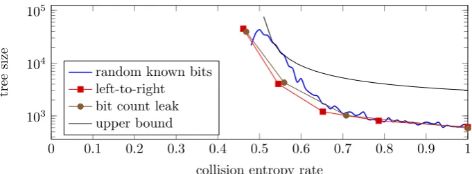
Figure 4: Validation of Theorem 3
Validation In order to empirically validate Theorem 3, we plot the predicted upper bound as well as the measured tree sizes in Figure 4, with pruning based on
• randomly known bits, similar to the setting of [4],
• left-to-right sliding window sequences of squares and multiply of varying window window width,
• a hypothetical leak where the attacker learns the number of set bits, but not their positions, per fixed window.
We find that the graph does not refute our theorem.
The graph measures the tree size for 50 randomly chosen 1024 bit keys. The search was aborted if the tree size exceeds 100,000 nodes. Note that close toH=0.5 and further left, the plots show the average search tree size over those attempts that finished within the limit.
Acknowledgments
We would like to thank all the other authors of [1, 2] for the opportunity to collaborate on this paper. This work was done while the author was affiliated with the University of Pennsylvania, with support from by the National Science Foundation under grants 1319880 and 14-519.
References
[2] Daniel J. Bernstein, Joachim Breitner, Daniel Genkin, Leon Groot Bruinderink, Nadia Heninger, Tanja Lange, Christine van Vredendaal, and Yuval Yarom. Sliding right into disaster: Left-to-right sliding windows leak. InCHES, volume 10529 ofLecture Notes in Computer Science, pages 555–576. Springer, 2017.
[3] Joachim Breitner and Maciej Skorski. Analytic formulas for renyi entropy of hidden markov models. CoRR, abs/1709.09699, 2017.
[4] Nadia Heninger and Hovav Shacham. Reconstructing RSA private keys from random key bits. InCRYPTO, volume 5677 ofLNCS, pages 1–17. Springer, 2009.
[5] Alfréd Rényi. On measures of entropy and information. InProceedings of the Fourth Berkeley Symposium on Mathematical Statistics and Probability, volume 1, pages 547–561, Berkeley, Calif., 1961.